Computer Vision is one of the hottest research fields within Deep Learning at the moment. It sits at the intersection of many academic subjects, such as Computer Science (Graphics, Algorithms, Theory, Systems, Architecture), Mathematics (Information Retrieval, Machine Learning), Engineering (Robotics, Speech, NLP, Image Processing), Physics (Optics), Biology (Neuroscience), and Psychology (Cognitive Science).

As Computer Vision represents a relative understanding of visual environments and their contexts, many scientists believe the field paves the way towards Artificial General Intelligence due to its cross-domain mastery.

So what is Computer Vision?

Here are a couple of formal textbook definitions:

• “the construction of explicit, meaningful descriptions of physical objects from images” (Ballard & Brown, 1982)
• “computing properties of the 3D world from one or more digital images” (Trucco & Verri, 1998)
• “to make useful decisions about real physical objects and scenes based on sensed images” (Sockman & Shapiro, 2001)

Why study Computer Vision?

The most obvious answer is that there’s a fast-growing collection of useful applications derived from this field of study. Here are just a handful of them:

• Face recognition: Snapchat and Facebook use face-detectionalgorithms to apply filters and recognize you in pictures.
• Image retrieval: Google Images uses content-based queries to search relevant images. The algorithms analyze the content in the query image and return results based on best-matched content.
• Gaming and controls: A great commercial product in gaming that uses stereo vision is Microsoft Kinect.
• Surveillance: Surveillance cameras are ubiquitous at public locations and are used to detect suspicious behaviors.
• Biometrics: Fingerprint, iris and face matching remains some common methods in biometric identification.
• Smart cars: Vision remains the main source of information to detect traffic signs and lights and other visual features.

I recently finished Stanford’s wonderful CS231n course on using Convolutional Neural Networks for visual recognition. Visual recognition tasks such as image classification, localization, and detection are key components of Computer vision.

Recent developments in neural networks and deep learning approaches have greatly advanced the performance of these state-of-the-art visual recognition systems. The course is a phenomenal resource that taught me the details of deep learning architectures being used in cutting-edge computer vision research. In this article, I want to share the 5 major computer vision techniques I’ve learned as well as major deep learning models and applications using each of them.

1 — Image Classification

The problem of image classification goes like this: Given a set of images that are all labeled with a single category, we’re asked to predict these categories for a novel set of test images and measure the accuracy of the predictions. There are a variety of challenges associated with this task, including viewpoint variation, scale variation, intra-class variation, image deformation, image occlusion, illumination conditions, and background clutter.

How might we go about writing an algorithm that can classify images into distinct categories? Computer Vision researchers have come up with a data-driven approach to solve this. Instead of trying to specify what every one of the image categories of interest look like directly in code, they provide the computer with many examples of each image class and then develop learning algorithms that look at these examples and learn about the visual appearance of each class.

In other words, they first accumulate a training dataset of labeled images, then feed it to the computer to process the data. Given that fact, the complete image classification pipeline can be formalized as follows:

• Our input is a training dataset that consists of N images, each labeled with one of K different classes.
• Then, we use this training set to train a classifier to learn what every one of the classes looks like.
• In the end, we evaluate the quality of the classifier by asking it to predict labels for a new set of images that it’s never seen before. We’ll then compare the true labels of these images to the ones predicted by the classifier.

The most popular architecture used for image classification is Convolutional Neural Networks (CNNs). A typical use case for CNNs is where you feed the network images and the network classifies the data. CNNs tend to start with an input “scanner” which isn’t intended to parse all the training data at once. For example, to input an image of 100 x 100 pixels, you wouldn’t want a layer with 10,000 nodes.

Rather, you create a scanning input layer of say 10 x 10 which you feed the first 10 x 10 pixels of the image. Once you passed that input, you feed it the next 10 x 10 pixels by moving the scanner one pixel to the right. This technique is known as sliding windows.

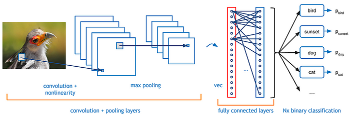
This input data is then fed through convolutional layers instead of normal layers. Each node only concerns itself with close neighboring cells. These convolutional layers also tend to shrink as they become deeper, mostly by easily divisible factors of the input. Besides these convolutional layers, they also often feature pooling layers. Pooling is a way to filter out details: a commonly found pooling technique is max pooling, where we take, say, 2 x 2 pixels and pass on the pixel with the most amount of a certain attribute.

Most image classification techniques nowadays are trained on ImageNet, a dataset with approximately 1.2 million high-resolution training images. Test images will be presented with no initial annotation (no segmentation or labels), and algorithms will have to produce labelings specifying what objects are present in the images. Some of the best existing computer vision methods were tried on this dataset by leading computer vision groups from Oxford, INRIA, and XRCE. Typically, computer vision systems use complicated multi-stage pipelines, and the early stages are typically hand-tuned by optimizing a few parameters.

The winner of the 1st ImageNet competition, Alex Krizhevsky (NIPS 2012), developed a very deep convolutional neural net of the type pioneered by Yann LeCun. Its architecture includes 7 hidden layers, not counting some max pooling layers. The early layers were convolutional, while the last 2 layers were globally connected. The activation functions were rectified linear units in every hidden layer. These train much faster and are more expressive than logistic units. In addition to that, it also uses competitive normalization to suppress hidden activities when nearby units have stronger activities. This helps with variations in intensity.

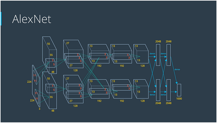
In terms of hardware requirements, Alex uses a very efficient implementation of convolutional nets on 2 Nvidia GTX 580 GPUs (over 1000 fast little cores). The GPUs are very good for matrix-matrix multiplies and also have very high bandwidth to memory. This allows him to train the network in a week and makes it quick to combine results from 10 patches at test time. We can spread a network over many cores if we can communicate the states fast enough. As cores get cheaper and datasets get bigger, big neural nets will improve faster than old-fashioned CV systems. Since AlexNet, there have been multiple new models using CNN as their backbone architecture and achieving excellent results in ImageNet: ZFNet (2013), GoogLeNet (2014), VGGNet (2014), ResNet (2015), DenseNet (2016) etc.

2 — Object Detection

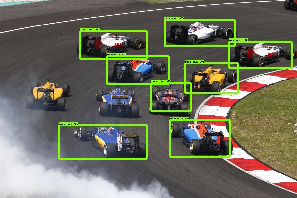
The task to define objects within images usually involves outputting bounding boxes and labels for individual objects. This differs from the classification / localization task by applying classification and localization to many objects instead of just a single dominant object. You only have 2 classes of object classification, which means object bounding boxes and non-object bounding boxes. For example, in car detection, you have to detect all cars in a given image with their bounding boxes.

If we use the Sliding Window technique like the way we classify and localize images, we need to apply a CNN to many different crops of the image. Because CNN classifies each crop as object or background, we need to apply CNN to huge numbers of locations and scales, which is very computationally expensive!

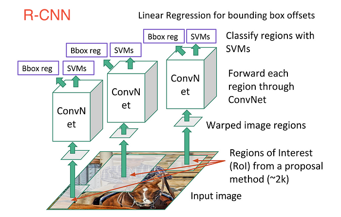
In order to cope with this, neural network researchers have proposed to use regions instead, where we find “blobby” image regions that are likely to contain objects.

This is relatively fast to run. The first model that kicked things off was R-CNN(Region-based Convolutional Neural Network). In a R-CNN, we first scan the input image for possible objects using an algorithm called Selective Search, generating ~2,000 region proposals. Then we run a CNN on top of each of these region proposals. Finally, we take the output of each CNN and feed it into an SVM to classify the region and a linear regression to tighten the bounding box of the object.

Essentially, we turned object detection into an image classification problem. However, there are some problems — the training is slow, a lot of disk space is required, and inference is also slow.

An immediate descendant to R-CNN is Fast R-CNN, which improves the detection speed through 2 augmentations: 1) Performing feature extraction before proposing regions, thus only running one CNN over the entire image, and 2) Replacing SVM with a softmax layer, thus extending the neural network for predictions instead of creating a new model.

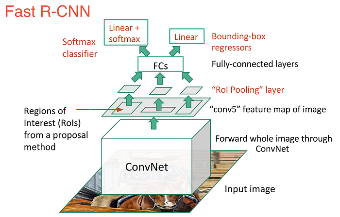
Fast R-CNN performed much better in terms of speed, because it trains just one CNN for the entire image. However, the selective search algorithm is still taking a lot of time to generate region proposals.

Thus comes the invention of Faster R-CNN, which now is a canonical model for deep learning-based object detection. It replaces the slow selective search algorithm with a fast neural network by inserting a Region Proposal Network (RPN) to predict proposals from features. The RPN is used to decide “where” to look in order to reduce the computational requirements of the overall inference process. The RPN quickly and efficiently scans every location in order to assess whether further processing needs to be carried out in a given region. It does that by outputting k bounding box proposals each with 2 scores representing the probability of object or not at each location.

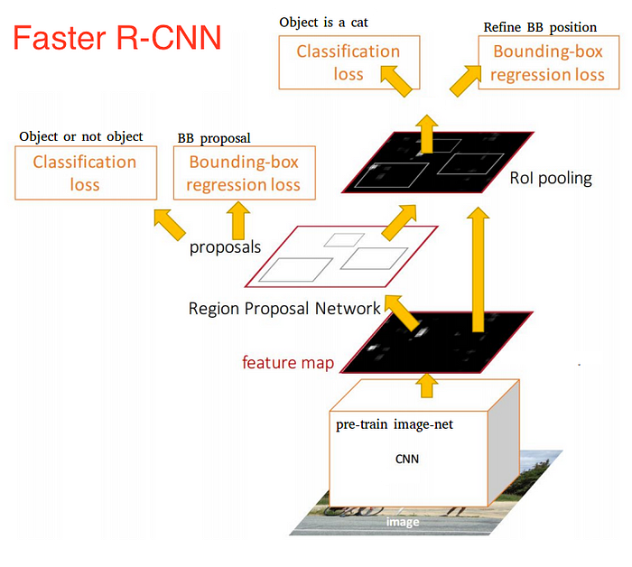
Once we have our region proposals, we feed them straight into what is essentially a Fast R-CNN. We add a pooling layer, some fully-connected layers, and finally a softmax classification layer and bounding box regressor.

Altogether, Faster R-CNN achieved much better speeds and higher accuracy. It’s worth noting that although future models did a lot to increase detection speeds, few models managed to outperform Faster R-CNN by a significant margin. In other words, Faster R-CNN may not be the simplest or fastest method for object detection, but it’s still one of the best performing.

Major Object Detection trends in recent years have shifted towards quicker, more efficient detection systems. This was visible in approaches like You Only Look Once (YOLO), Single Shot MultiBox Detector (SSD), and Region-Based Fully Convolutional Networks (R-FCN) as a move towards sharing computation on a whole image. Hence, these approaches differentiate themselves from the costly subnetworks associated with the 3 R-CNN techniques. The main rationale behind these trends is to avoid having separate algorithms focus on their respective subproblems in isolation, as this typically increases training time and can lower network accuracy.

3 — Object Tracking

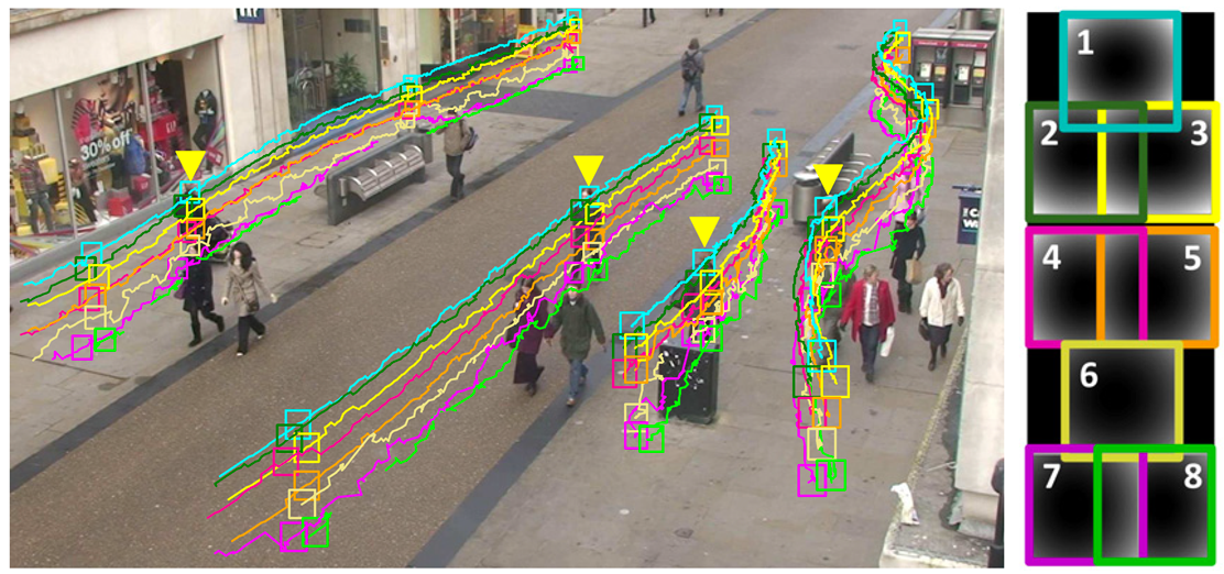
Object Tracking refers to the process of following a specific object of interest, or multiple objects, in a given scene. It traditionally has applications in video and real-world interactions where observations are made following an initial object detection. Now, it’s crucial to autonomous driving systems such as self-driving vehicles from companies like Uber and Tesla.

Object Tracking methods can be divided into 2 categories according to the observation model: generative method and discriminative method. The generative method uses the generative model to describe the apparent characteristics and minimizes the reconstruction error to search the object, such as PCA.

The discriminative method can be used to distinguish between the object and the background, its performance is more robust, and it gradually becomes the main method in tracking. The discriminative method is also referred to as Tracking-by-Detection, and deep learning belongs to this category. To achieve tracking-by-detection, we detect candidate objects for all frames and use deep learning to recognize the wanted object from the candidates. There are 2 kinds of basic network models that can be used: stacked auto encoders (SAE) and convolutional neural network (CNN).

The most popular deep network for tracking tasks using SAE is Deep Learning Tracker, which proposes offline pre-training and online fine-tuning the net. The process works like this:

• Off-line unsupervised pre-train the stacked denoising auto-encoder using large-scale natural image datasets to obtain the general object representation. Stacked denoising auto-encoder can obtain more robust feature expression ability by adding noise in input images and reconstructing the original images.
• Combine the coding part of the pre-trained network with a classifier to get the classification network, then use the positive and negative samples obtained from the initial frame to fine-tune the network, which can discriminate the current object and background. DLT uses particle filter as the motion model to produce candidate patches of the current frame. The classification network outputs the probability scores for these patches, meaning the confidence of their classifications, then chooses the highest of these patches as the object.
• In the model updating, DLT uses the way of limited threshold.

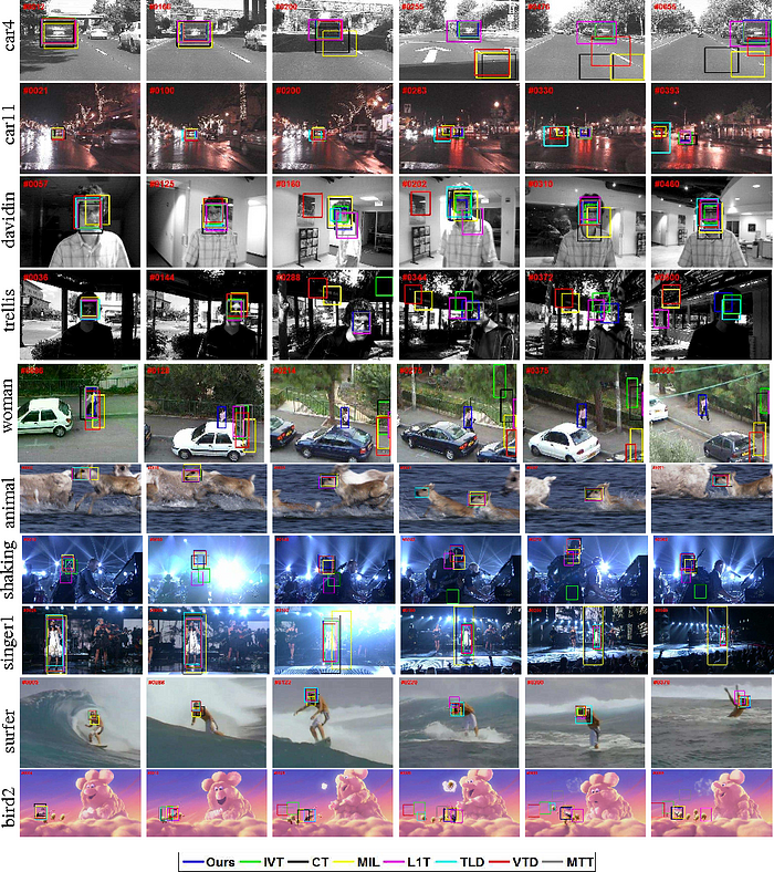
Because of its superiority in image classification and object detection, CNN has become the mainstream deep model in computer vision and in visual tracking. Generally speaking, a large-scale CNN can be trained both as a classifier and as a tracker. 2 representative CNN-based tracking algorithms are fully-convolutional network tracker (FCNT) and multi-domain CNN (MD Net).

FCNT analyzes and takes advantage of the feature maps of the VGG modelsuccessfully, which is a pre-trained ImageNet, and results in the following observations:

• CNN feature maps can be used for localization and tracking.
• Many CNN feature maps are noisy or un-related for the task of discriminating a particular object from its background.
• Higher layers capture semantic concepts on object categories, whereas lower layers encode more discriminative features to capture intra-class variation.

Because of these observations, FCNT designs the feature selection network to select the most relevant feature maps on the conv4–3 and conv5–3 layers of the VGG network. Then in order to avoid overfitting on noisy ones, it also designs extra two channels (called SNet and GNet) for the selected feature maps from two layers’ separately. The GNet captures the category information of the object, while the SNet discriminates the object from a background with a similar appearance.

Both of the networks are initialized with the given bounding-box in the first frame to get heat maps of the object, and for new frames, a region of interest (ROI) centered at the object location in the last frame is cropped and propagated. At last, through SNet and GNet, the classifier gets two heat maps for prediction, and the tracker decides which heat map will be used to generate the final tracking result according to whether there are distractors. The pipeline of FCNT is shown below.

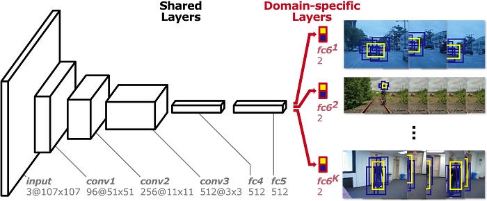
Different from the idea of FCNT, MD Net uses all the sequences of a video to to track movements in them. The networks mentioned above use irrelevant image data to reduce the training demand of tracking data, and this idea has some deviation from tracking. The object of one class in this video can be the background in another video, so MD Net proposes the idea of multi-domain to distinguish the object and background in every domain independently. And a domain indicates a set of videos that contain the same kind of object.

As shown below, MD Net is divided into 2 parts: the shared layers and the K branches of domain-specific layers. Each branch contains a binary classification layer with softmax loss, which is used to distinguish the object and background in each domain, and the shared layers sharing with all domains to ensure the general representation.

In recent years, deep learning researchers have tried different ways to adapt to features of the visual tracking task. There are many directions that have been explored: applying other network models such as Recurrent Neural Netand Deep Belief Net, designing the network structure to adapt to video processing and end-to-end learning, optimizing the process, structure, and parameters, or even combining deep learning with traditional methods of computer vision or approaches in other fields such as Language Processingand Speech Recognition.

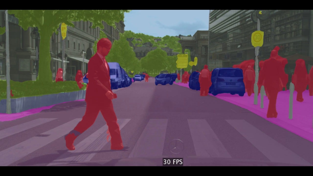
Central to Computer Vision is the process of segmentation, which divides whole images into pixel groupings which can then be labelled and classified.

Particularly, Semantic Segmentation tries to semantically understand the role of each pixel in the image (e.g. is it a car, a motorbike, or some other type of class?). For example, in the picture above, apart from recognizing the person, the road, the cars, the trees, etc., we also have to delineate the boundaries of each object. Therefore, unlike classification, we need dense pixel-wise predictions from our models.

As with other computer vision tasks, CNNs have had enormous success on segmentation problems. One of the popular initial approaches was patch classification through a sliding window, where each pixel was separately classified into classes using a patch of images around it. This, however, is very inefficient computationally because we don’t reuse the shared features between overlapping patches.

The solution, instead, is UC Berkeley’s Fully Convolutional Networks (FCN), which popularized end-to-end CNN architectures for dense predictions without any fully connected layers. This allowed segmentation maps to be generated for images of any size and was also much faster compared to the patch classification approach. Almost all subsequent approaches to semantic segmentation adopted this paradigm.

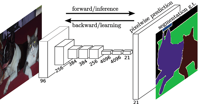
However, one problem remains: convolutions at original image resolution will be very expensive. To deal with this, FCN uses downsampling and upsampling inside the network. The downsampling layer is known as striped convolution, while the upsampling layer is known as transposed convolution.

Despite the upsampling/downsampling layers, FCN produces coarse segmentation maps because of information loss during pooling. SegNet is a more memory efficient architecture than FCN that uses-max pooling and an encoder-decoder framework. In SegNet, shortcut/skip connections are introduced from higher resolution feature maps to improve the coarseness of upsampling/downsampling.

Recent research in Semantic Segmentation all relies heavily on fully convolutional networks, such as Dilated Convolutions, DeepLab, and RefineNet.

5 — Instance Segmentation

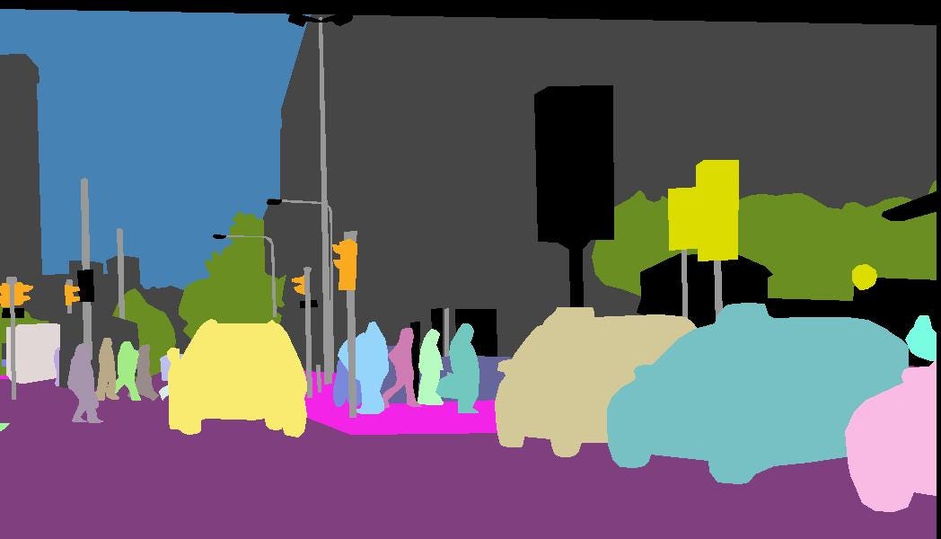
Beyond Semantic Segmentation, Instance Segmentation segments different instances of classes, such as labelling 5 cars with 5 different colors. In classification, there’s generally an image with a single object as the focus and the task is to say what that image is. But in order to segment instances, we need to carry out far more complex tasks. We see complicated sights with multiple overlapping objects and different backgrounds, and we not only classify these different objects but also identify their boundaries, differences, and relations to one another!

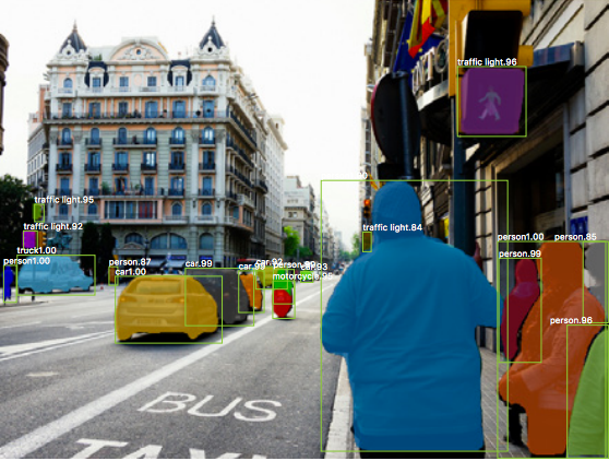
So far, we’ve seen how to use CNN features in many interesting ways to effectively locate different objects in an image with bounding boxes. Can we extend such techniques to locate exact pixels of each object instead of just bounding boxes? This instance segmentation problem is explored at Facebook AI using an architecture known as Mask R-CNN.

Much like Fast R-CNN, and Faster R-CNN, Mask R-CNN’s underlying intuition is straightforward Given that Faster R-CNN works so well for object detection, could we extend it to also carry out pixel-level segmentation?

Mask R-CNN does this by adding a branch to Faster R-CNN that outputs a binary mask that says whether or not a given pixel is part of an object. The branch is a Fully Convolutional Network on top of a CNN-based feature map. Given the CNN Feature Map as the input, the network outputs a matrix with 1s on all locations where the pixel belongs to the object and 0s elsewhere (this is known as a binary mask).

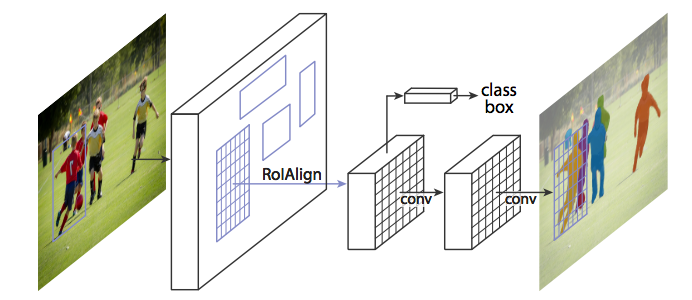
Additionally, when run without modifications on the original Faster R-CNN architecture, the regions of the feature map selected by RoIPool (Region of Interests Pool) were slightly misaligned from the regions of the original image. Since image segmentation requires pixel-level specificity, unlike bounding boxes, this naturally led to inaccuracies. Mask R-CNN solves this problem by adjusting RoIPool to be more precisely aligned using a method known as RoIAlign (Region of Interests Align). Essentially, RoIAlign uses bilinear interpolation to avoid error in rounding, which causes inaccuracies in detection and segmentation.

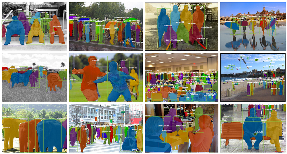
Once these masks are generated, Mask R-CNN combines them with the classifications and bounding boxes from Faster R-CNN to generate such wonderfully precise segmentations:

Conclusion

These 5 major computer vision techniques can help a computer extract, analyze, and understand useful information from a single or a sequence of images. There are many other advanced techniques that I haven’t touched, including style transfer, colorization, action recognition, 3D objects, human pose estimation, and more.

Indeed, the field of Computer Vision is too expensive to cover in depth, and I would encourage you to explore it further, whether through online courses, blog tutorials, or formal documents. I’d highly recommend CS231n for starters, as you’ll learn to implement, train, and debug your own neural networks. As a bonus, you can get all the lecture slides and assignment guidelines from my GitHub repository. I hope it’ll guide you in the quest of changing how to see the world!

If you enjoyed this piece, I’d love it if you hit the clap button 👏 so others might stumble upon it. You can find my own code on GitHub, and more of my writing and projects at https://jameskle.com/. You can also follow me on Twitter, email me directly or find me on LinkedIn. Sign up for my newsletter to receive my latest thoughts on data science, machine learning, and artificial intelligence right at your inbox!

Discuss this post on Hacker News.