Introduction

Speech recognition is invading our lives. It’s built into our phones (Siri), our game consoles (Kinect), our smartwatches (Apple Watch), and even our homes (Amazon Echo). But speech recognition has been around for decades, so why is it just now hitting the mainstream?

The reason is that deep learning finally made speech recognition accurate enough to be useful outside of carefully-controlled environments. In this blog post, we’ll learn how to perform speech recognition with 3 different implementations of popular deep learning frameworks.

Note: The content of this blog post comes from Navdeep Jaitly’s lecture at Stanford. I’d highly recommend watching his talk for the full details.

Speech Recognition — The Classic Way

In the era of OK Google, I might not really need to define ASR, but here’s a basic description: Say you have a person or an audio source saying something textual, and you have a bunch of microphones that are receiving the audio signals. You can get these signals from one or many devices, and then pass them into an ASR system — whose job it is to infer the original source transcript that the person spoke or that the device played.

So why is ASR important?

Firstly, it’s a very natural interface for human communication. You don’t need a mouse or a keyboard, so it’s obviously a good way to interact with machines. You don’t even really need to learn new techniques because most people learn to speak as a function of natural development. It’s a very natural interface for talking with simple devices such as cars, handheld phones, and chatbots.

So how is this done classically?

As observed above, the classic way of building a speech recognition system is to build a generative model of language. On the rightmost side, you produce a certain sequence of words from language models. And then for each word, you have a pronunciation model that says how this particular word is spoken. Typically it’s written out as the sequence of phonemes — which are basic units of sound, but for our vocabulary, we’ll just say a sequence of tokens — which represent a cluster of things that have been defined by linguistics experts.

Then, the pronunciation models are fed into an acoustic model, which basically defines how does a given token sounds. These acoustic models are now used to describe the data itself. Here the data would be x, which is the sequence of frames of audio features from x1 to xT. Typically, these features are something that signal processing experts have defined (such as the frequency components of the audio waveforms that are captured).

Each of these different components in this pipeline uses a different statistical model:

• In the past, language models were typically N-gram models, which worked very well for simple problems with limited speech input data. They are essentially tables describing the probabilities of token sequences.
• The pronunciation models were simple lookup tables with probabilities associated with pronunciations. These tables would be very large tables of different pronunciations.
• Acoustic models are built using Gaussian Mixture Models with very specific architectures associated with them.
• The speech processing was pre-defined.

Once we have this kind of model built, we can perform the recognition by doing the inference on the data received. So you get a waveform, you compute the features for it (X) and do a search for Y that gives the highest probabilities of X.

The Neural Network Invasion

Over time, researchers started noticing that each of these components could work more effectively if we used neural networks.

• Instead of the N-gram language models, we can build neural language models and feed them into a speech recognition system to restore things that were produced by a first path speech recognition system.
• Looking into the pronunciation models, we can figure out how to do pronunciation for a new sequence of characters that we’ve never seen before using a neural network.
• For acoustic models, we can build deep neural networks (such as LSTM-based models) to get much better classification accuracy scores of the features for the current frame.
• Interestingly enough, even the speech pre-processing steps were found to be replaceable with convolutional neural networks on raw speech signals.

However, there’s still a problem. There are neural networks in each component, but they’re trained independently with different objectives. Because of that, the errors in one component may not behave well with the errors in another component. So that’s the basic motivation for devising a process where you can train the entire model as one big component itself.

These so-called end-to-end models encompass more and more components in the pipeline discussed above. The 2 most popular ones are (1) Connectionist Temporal Classification (CTC), which is in wide usage these days at Baidu and Google, but it requires a lot of training; and (2) Sequence-To-Sequence (Seq-2-Seq), which doesn’t require manual customization.

The basic motivation is that we want to do end-to-end speech recognition. We are given the audio X — which is a sequence of frames from x1 to xT, and the corresponding output text Y — which is a sequence of y1 to yL. Y is just a text sequence (transcript) and X is the audio processed spectrogram. We want to perform speech recognition by learning a probabilistic model p(Y|X): starting with the data and predicting the target sequences themselves.

1 — Connectionist Temporal Classification

The first of these models is called Connectionist Temporal Classification (CTC) ([1], [2], [3]). X is a sequence of data frames with length T: x1, x2, …, xT, and Y is the output tokens of length L: y1, y2, …, yL. Because of the way the model is constructed, we require T to be greater than L.

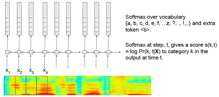
This model has a very specific structure that makes it suitable for speech:

• You get the spectrogram at the bottom (X). You feed it into a bi-directional recurrent neural network, and as a result, the arrow pointing at any time step depends on the entirety of the input data. As such, it can compute a fairly complicated function of the entire data X.
• This model, at the top, has softmax functions at every timeframe corresponding to the input. The softmax function is applied to a vocabulary with a particular length that you’re interested in. In this case, you have the lowercase letters a to z and some punctuation symbols. So the vocabulary for CTC would be all that and an extra token called a blank token.
• Each frame of the prediction is basically producing a log probability for a different token class at that time step. In the case above, a score s(k, t) is the log probability of category k at time step t given the data X.

In a CTC model, if you look at just the softmax functions that are produced by the recurring neural network over the entire time step, you’ll be able to find the probability of the transcript through these individual softmax functions over time.

Let’s take a look at an example (below). The CTC model can represent all these paths through the entire space of softmax functions and look at only the symbols that correspond to each of the time steps.

As seen on the left, the CTC model will go through 2 C symbols, then through a blank symbol, then produce 2 A symbols, then produce another blank symbol, then transition to a T symbol, and then finally produce a blank symbol again.

So when you go through these paths with the constraint, you can only transition between the same phoneme from one step to the next. Therefore, you’ll end up with different ways of representing an output sequence.

For the example above, we have cc <b> aa <b> t <b> or cc <b> <b> a <b> t <b> or cccc <b> aaaa <b> tttt <b>. Given these constraints, it turns out that even though there’s an exponential number of paths by which you can produce the same output symbol, you can actually do it correctly using a dynamic programming algorithm. Because of dynamic programming, it’s possible to compute both the log probability p(Y|X) and its gradient exactly. This gradient can be backpropagated to a neural network whose parameters can then be adjusted by your favorite optimizer!

Below are some results for CTC, which show how the model functions on given audio. A raw waveform is aligned at the bottom, and the corresponding predictions are outputted at the top. You can see that it produces the symbol H at the beginning. At a certain point, it gets a very high probability, which means that the model is confident that it hears the sound corresponding to H.

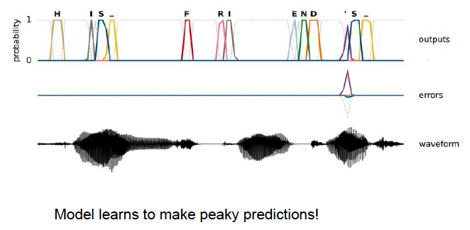
However, there are some drawbacks to CTC language models. They often misspell words and struggle with grammar. So if you had some way to figure out how to rank the different paths produced from the model and re-rank them just by the language model, the results should be much better.

Google actually fixed these problems by integrating a language model as part of the CTC model itself during training. That’s the kind of production model currently being deployed with OK Google.

2 — Sequence-To-Sequence

An alternative approach to speech processing is the sequence-to-sequence model that makes next-step predictions. Let’s say that you’re given some data X and that you need to produce some symbols y1 to y{i}. The model predicts the probability of the next symbol of y{i+1}. The goal here is to basically learn a very good model for p.

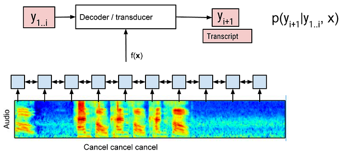
With the model architecture (left), you have a neural network (which is the decoder in a sequence-to-sequence model) that looks at the entire input (which is the encoder). It feeds in the path symbols that are produced as a recurrent neural network, and then you predict the next token itself as the output.

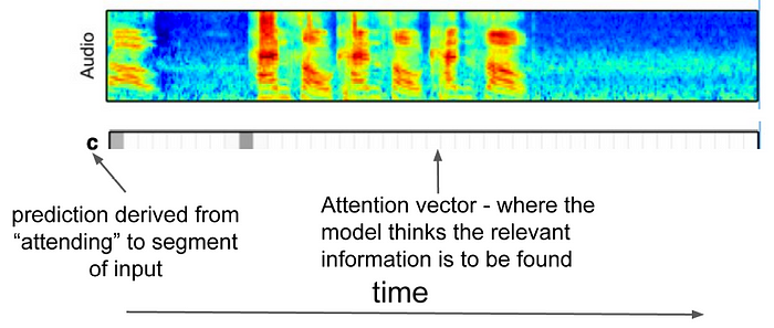
So this model does speech recognition with the sequence-to-sequence framework. In translation, the X would be the source language. In the speech domain, the X would be a huge sequence of audio that’s now encoded with a recurrent neural network.

What it needs to function is the ability to look at different parts of temporal space, because the input is really long. Intuitively, translation results get worse as the source sentence becomes longer. That’s because it’s really difficult for the model to look in the right place. Turns out, that problem is aggravated a lot more with audio streams that are much longer. Therefore, you would need to implement an attention mechanism if you want to make this model work at all.

Seen in the example on the left, you’re trying to produce the 1st character C. You create an attention vector that essentially looks at different parts of the input time steps and produces the next chapter (which is A) after changing the attention.

If you keep doing this over the entire input stream, then you’re moving forward attention just learned by the model itself. Seen here, it produces the output sequence “cancel, cancel, cancel.”

The Listen, Attend, and Spell [4] model is the canonical model for the seq-2-seq category. Let’s look at the diagram below taken from the paper:

• In the Listener architecture, you have an encoder structure. For every time step of the input, it produces a vector representation that encodes the input and is represented as h_t at time step t.
• In the Speller architecture, you have a decoder architecture. You generate the next character c_t at every time step t.
• The LAS model uses a hierarchical encoder to replace the traditional recurrent neural network. Instead of processing one frame for every time step, it collapses neighboring frames as you feed into the next layer. Because of that, it reduces the number of time steps to be processed, thus making the processing faster.

So what are the limitations of this model?

• One of the big limitations preventing its use in an online system is that the output produced is being conditioned on the entire input. That means if you’re going to put the model in a real-world speech recognition system, you’d have to first wait for the entire audio to be received before outputting the symbol.
• Another limitation is that the attention model itself is a computational bottleneck since every output token pays attention to every input time step. This makes it harder and slower for the model to do its learning.
• Further, as the input is received and becomes longer, the word error rate goes down.

3 — Online Sequence-to-Sequence

Online sequence-to-sequence models are designed to overcome the limits of sequence-to-sequence models—you don’t want to wait for the entire input sequence to arrive, and you also want to avoid using the attention model itself over the entire sequence. Essentially, the intention is to produce the outputs as the inputs arrive. It has to solve the following problem: is the model ready to produce an output now that it’s received this much input?

The most notable online seq-2-seq model is called a Neural Transducer [5]. If you take the input as it comes in, and every so often at a regular interval, you can run a seq-2-seq model on what’s been received in the last block. As seen in the architecture below, the encoder’s attention (instead of looking at the entire input) will focus only on a little block. The transducer will produce the output symbols.

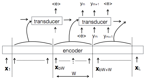
The nice thing about the neural transducer is that it maintains causality. More specifically, the model preserves the disadvantage of a seq-2-seq model. It also introduces an alignment problem: in essence, what you want to know is that you have to produce some symbols as outputs, but you don’t know which chunk these symbols should be aligned to.

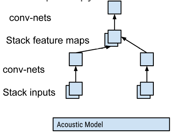
You can actually make this model better by incorporating convolutional neural networks, which are borrowed from computer vision. The paper [6] uses CNNs to do the encoder side in speech architecture.

You take the traditional model for the pyramid as seen to the left, and instead of building the pyramid by simply stacking 2 things together, you can put a fancy architecture on top when you do the stacking. More specifically, as seen below, you can stack them as feature maps and put a CNN on the top. For the speech recognition problem, the frequency bands and the timestamps of the features that you look at will correspond to a natural substructure of the input data. The convolutional architecture essentially looks at that substructure.

Conclusion

You should now generally be up to speed on the 3 most common deep learning-based frameworks for performing automatic speech recognition in a variety of contexts. The papers that I’ve referenced below will help you get into the nitty-gritty technical details of how they work if you’re inclined to do that.

References

[1] Graves, Alex, and Navdeep Jaitly. “Towards End-To-End Speech Recognition with Recurrent Neural Networks.” ICML. Vol. 14. 2014.

[2] Amodei, Dario, et al. “Deep speech 2: End-to-end speech recognition in english and mandarin.” arXiv preprint arXiv:1512.02595 (2015).

[3] H. Sak, A. Senior, K. Rao, O. Irsoy, A. Graves, F. Beaufays, and J. Schalkwyk, “Learning acoustic frame labeling for speech recognition with recurrent neural networks,” in IEEE International Conference on Acoustics, Speech, and Signal Processing (ICASSP), 2015.

[4] W. Chan, N. Jaitly, Q. Le, and O. Vinyals. “Listen, Attend, and Spell,” in IEEE International Conference on Acoustics, Speech, and Signal Processing (ICASSP), 2015.

[5] N. Jaitly, D. Sussillo, Q. Le, O. Vinyals, I. Sutskever, and S. Bengio. “A Neural Transducer,” arXiv preprint arXiv:1511.04868 (2016).

[6] N. Jaitly, W. Chan, and Y. Zhang. “Very Deep Convolutional Networks for End-to-End Speech Recognition,” arXiv preprint arXiv:1610.03022 (2016).