Authors: Drake Johnson (drakej@stanford.edu), Tim Ngo (ngotm@stanford.edu), Augusto Fernandez (afyrxr@stanford.edu)
I. Introduction:
Recently, there has been an increase in interest in the public for the ecosystem surrounding humans. Often, it is believed that a deeper understanding of the ecological context one lives in makes them more likely to advocate for environmental activism, and because of this, it is important to cultivate this increased interest. In spite of this, it is sometimes difficult to learn more about the ecosystem around a location without expert help, especially when one does not have the specific vocabulary to describe the ecosystem.
One way to ameliorate this is by providing the climate classification for a specific image. Although climate is not the only variable that characterizes an ecosystem, it is a simple piece of information that provides a jumping off point to learn more about the natural world in general. Furthermore, with the rise of global warming, climate is an important aspect of the system, as different climates may change drastically in the future. Finally, climate is a practical choice for public education, as systems such as the Köppen-Geiger climate classifications are well structured and defined.
We want to create a tool to recognize climate category based on photos. With this, one could take a picture of the nature they may be around, and immediately know what ecosystem they are actively affecting. Instead of an abstract idea, the ecosystem will then be tangible. Furthermore, this could serve as a general educational tool, allowing people to be more familiar with images of ecosystems they may stumble across. The classifier takes in an image of a natural landscape as input and outputs the climate that is most likely shown in the picture. In this work, we use several different machine learning paradigms to attempt to achieve this aim, with best performance using a ResNet Convolutional Neural Network.
II. Related Work
Most work done on climate classification thus far seems to be focused on using satellite imagery or multi-spectral data as opposed to landscape imagery of photos taken from Earth. Generally these projects employed SVMs or random forests (RFs) to perform the classification.
A project in South Africa used imagery from the RapidEye satellite to classify tree species in semi-arid areas [1]. An analysis for classifying different agricultural landscapes employed both RFs and SVMs but found no statistically significant difference between them [2]. A project that was specifically focused on urban climates evaluated SVMs, RFs and a neural network to identify urban climates from satellite imagery and in particular, accuracy of 97.4% and 95.3% was achieved on the neural network and RF respectively [3]. Additionally, another project studied different statistical methods for ecological classification and found that RFs performed better when compared to logistic regression and other common methods [4].
Because most projects already out there seem to focus on using satellite imagery or advanced data to perform climate classification, we decided that it would be best to use landscape imagery taken by people on Earth as this would make the use of our project more readily accessible to a common user.
We did find that a similar project used street view or user taken images and attempted to identify from where the images were taken [5]. Instead of using regression to predict latitude and longitude, the surface of the earth into cells in order to cast geolocation as a classification problem, and the probability that a given image was taken in each cell was predicted using convolutional neural networks. It was found that the model outperformed image retrieval methods more commonly used for geolocation, sometimes even achieving “superhuman” accuracy [5]. The high accuracy of this project made it seem feasible for us to take on the project we chose. Furthermore because of the success that a convolutional neural network model exhibited both in this study and the urban climate study we decided to use a CNN in our project as well.
III. Dataset and Features
To acquire training and testing data we started by identifying a dataset of publicly available Flickr images that were geotagged [6]. We then built a script to filter through the images in this dataset, based on user-provided tags. In particular, we were focused mainly on nature and landscape images for this project and we tried to eliminate photos of people or urban shots. Flickr provides users with the option to tag images with keywords. This allowed us to select images with keywords relevant to landscapes, and filter out undesirable images, such as portraits and street photography. Desired tags included “landscape,” “outdoors” and “nature,” while undesired tags included, “urban,” “me,” “portrait” and “nyc,” among others. We then downloaded the subset of images that satisfied the required filters. This gave us a total of about 320,000 images, mostly of natural landscapes, to work with. Due to the tags being user-provided, however, some images did not depict landscapes, resulting in noisy labels. Nevertheless, mapping the geolocations of our dataset show that we have representative images of climates from most of the world.

For the class labels we initially used the Köppen climate classification system but found that many of the climates were severely overshadowed by other climates with many more representative images in our dataset. As such we grouped certain Köppen climates together and came up with our own broader classification system for the climates. The thirteen overarching classes and the Köppen climates they represent are listed below in Table 1. Using all 320,000 images, however, ended up being too computationally demanding for our resources. Because of this, we decided to only use a sample of our initial dataset. Certain climates, such as oceanic, had many more images attributed to them, resulting in a relative class imbalance, so in downsampling, we chose to sample the same number of images from each climate, which balanced the classes. We felt this was reasonable, as although the results are not representative of our models performance on the original dataset, the model is not intended to be used on the original dataset, but rather user inputted images.
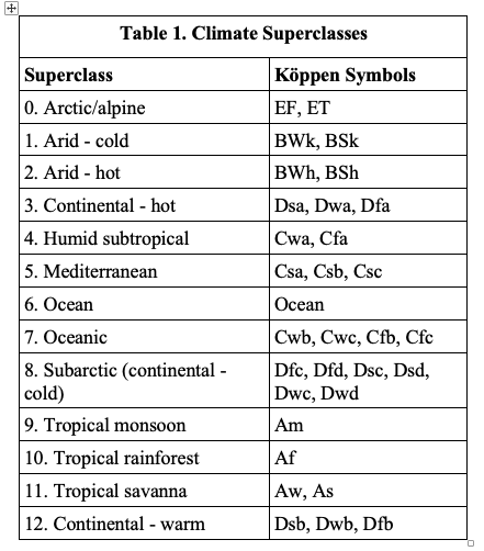
The images were then labelled using their latitude and longitude metadata and Köppen-Geiger climate classification map data [7], by finding the nearest geolocation to the image metadata in the climate map.
We then pre-processed the images to make them a uniform size and have a more manageable number of pixels. After resizing every image to 224 by 224 pixels (with 3 color channels), the pixel values were then normalized to be standard normal.
An analysis of our final dataset showed a reasonable spread of locations across the world, as well as across different climates. Because we manually balanced our classes, we also see even numbers of climates in our dataset. Finally, we randomly split our dataset and stratified to maintain class balances, setting 60% for training, 20% for validation, and 20% for testing.
IV. Methods
In order to establish a baseline for performance of a model on our dataset, we trained a logistic regression model and a support vector machine model. After an initial attempt to train these models on normalized pixel values, we decided to manually create features from the images first. This could reduce the dimensionality of the features, and create more tractable information. To do this, we used Histograms of Oriented Gradients (HOG). HOG was used both for its computational efficiency and its use in image classification in the literature, although not tested on landscape imagery specifically [12]. HOG works by calculating several different orders of gradients over the image, and then calculating frequencies of these gradients in grids across the image. After tuning parameters, the best performing version of this algorithm resulting in a 1,568 dimensional feature vector, which was then normalized to have mean 0 and standard deviation of 1.
With these features, we then train a logistic regression classifier. Logistic regression models the relationship between features and the response variable, which in this case is the climate, through the logistic function, which takes the form:

X is the features corresponding to a given image, and θ is the parameter that our model learns during training. This outputs a vector with values for each climate, which we then get our prediction from by taking the softmax of this vector. To optimize this parameter, we perform l2 regularization by minimizing the following cost function:

where C is the regularization term.
We found, however, that when training the model on our derived features, we achieved 100% accuracy on the training data. Upon inspection, we realized that there were more dimensions in our feature vector than there were training examples, and thus the model matrix was not full rank. To account for this, we used only the first one hundred principal components of each feature, transforming each feature using principal component analysis (PCA). PCA finds orthogonal components that describe the most variation within the data, which each vector can then be projected onto.
We then trained an SVM model to get another baseline accuracy. SVM works by maximizing the cost function:

subject to the constraint that

with

where <x (i), x (j)> is given by some kernel function K. By doing this, the algorithm finds a hyperplane that optimally separates two classes of data, by maximizing the minimum distance between data points and the plane. However, because we have more than two classes of data, we use a one vs one paradigm, creating many different models to account for each pairing of classes.
Finally, to tune the hyperparameters, we perform a grid search over regularization constants for linear regression and kernels for SVM, using 3 fold cross validation on the training data.
After having our two baselines we proceeded to try and build a more robust model using a convolutional neural network. In particular, we selected the ResNet-18 architecture. This residual neural network consists of an initial convolutional layer, 8 two-layer ResNet blocks and a final fully connected layer. Furthermore, we used a transfer learning approach. A ResNet was pre-trained on the ImageNet dataset, yielding high performance classification for general images. Theoretically, this allows the hidden layers of the model to already know useful features about images already.
We then take this model and modify the output and input layer for our specific classification task. We also normalize each image to a predefined mean and variance, both slightly above 0, given by the initial dataset [13]. Finally, we retune the model from these starting weights on our own dataset through standard back propagation, using a loss function of cross-entropy. We found convergence of loss after training for 30 epochs, using .001 for a learning rate, a mini-batch size of 64, and momentum of .9 to avoid local minima. These parameters were chosen through manual tuning to minimize validation loss, due to computational limitations to searching across a larger search space.
Each residual block contains a shortcut connection, by way of adding the outputs before the block, x, to the outputs of the stacked layers, F(x), as shown in Figure 2. The addition of the identity is hypothesized to facilitate optimization by making it straightforward for a layer to become an identity mapping, by allowing F(x) to go to zero [8]. This effectively allows deep models to behave more like shallower models when doing so is more optimal.

V. Experiments/Results/Discussion
To analyze our results, we primarily care about accuracy, given simply by the correct number of classifications over the total number of classifications. This is because false positives and false negatives are equivalent to us, and need not be weighed differently.
Our baselines did not perform accurately but this is to be expected. Below is a graph of the first three components from a PCA of the histogram of gradients features:
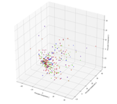
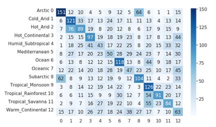
As can be seen, these classes are not obviously separable in this dimension, although the first three components were only shown to explain 20% of the variation in our features, and may still be separable in higher dimension. Clearly climate classification is something very nuanced and hard to distinguish with the given features. Indeed in the confusion matrix for logistic regression on the test set we see poor performance.
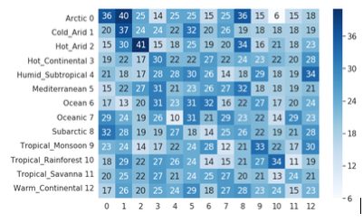
Our overall accuracies for the logistic regression model were 0.27 on the training set and then 0.13 and 0.1 respectively on the validation and testing sets. Seeing as we have 13 superclasses we see that the logistic regression model performed only slightly better than chance.
The SVM model also performed poorly, although better than logistic regression. While during training we achieved an accuracy of 0.77, during validation and testing we achieved an accuracy of only 0.12 and 0.15 respectively. The confusion matrix for the performance of SVM on the testing set is reported below.
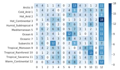
The CNN performed better than we expected. As can be seen from the confusion matrix, even when predicting incorrectly, the predicted classes were often closely related to the true class. The three tropical climates were often conflated with each other, arctic and subarctic climates were linked, and the two arid climates were linked as well.
To better interpret errors made by our CNN model, we mapped class activations for selected images. This allows us to visualize the implicit “focus” of the CNN on different regions of an image [9].
As seen in Figure 7, when classifying the above image as a rainforest, the CNN was indeed focusing on the trees on the island, whereas the focus for subarctic was on the sea while ignoring the island. It is likely that that particular shade of blue appears often in subarctic photos and that’s what led to the model finding that label as well.
The table below summarizes the overall performance of each model
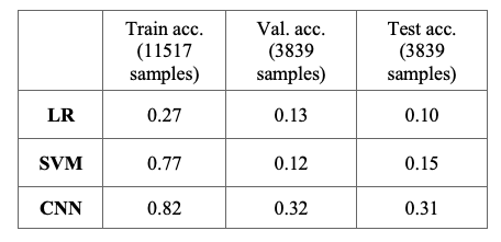
Figure 7. CAM for “Tropical Rainforest” (top) and “Subartic” (bottom)
VI. Conclusions/Future Work
There are numerous aspects of the project we feel we could’ve improved upon given more time. To start with, we would have liked to better curate the dataset. Because we relied upon an initial set of Flickr images with user-entered labels to classify them as landscape, nature, etc. we ended up with some noise in our dataset. While we did our best to filter out these noisy images, inevitably some went through and we ended up with images of interiors or shots that are not relevant for climate classification. Ideally the database we train on should include only nature shots.
We also had to tag these images with a specific label from our 13 superclasses using their GPS coordinates. Ideally we could come up with a better proxy for climate when labelling our dataset which would again serve the purpose of leading to less noise or inaccuracies within the data itself.
Furthermore, while currently our model only takes into account the raw pixel values of the image itself. We foresee that improvements could be made by also using the season during which the photo was taken as a feature. Landscapes can look very different depending on the time of year and this is something that we saw is causing misclassifications with our model in its current state. In general, snowed on landscapes are being classified as arctic or subarctic.
VII: Code
Github: https://github.com/timmngo/cs229-koppen
Google Drive: https://drive.google.com/file/d/1ODVCH2_dG5NMV012Jd1j09lq8UF9viib/view?usp=sharing
VIII: Contributions
All
● Worked on proposal, milestone, poster, and report, and collaborated on coding
● Met often to work together in-person
● Experimented with different parameters/models and documented results
Drake Johnson (drakej@stanford.edu)
● Set up notebooks for our LR, SVM, and CNN experiments
● Set up VM instance/programming environment
● Performed principal component analysis
Tim Ngo (ngotm@stanford.edu)
● Set up notebook for class activation mapping
● Worked on scripts to filter, label, and download images from the dataset
Augusto Fernández (afytxr@stanford.edu)
● Contributed significantly to milestone and final report
● Worked on scripts to filter, label, and download images from the dataset
IX. REFERENCES
[1] S. Adelabu, O. Mutanga, E. E. Adam, M. A. Cho, “Exploiting machine learning algorithms for tree species classification in a semiarid woodland using RapidEye image,” J. Appl. Rem. Sens. 7(1) 073480, Nov. 2013. https://www.spiedigitallibrary.org/journalArticl e/Download?fullDOI=10.1117%2F1.JRS.7.073 480
[2] D. C. Duro, S. E. Franklin, M. G. Dubé, “A comparison of pixel-based and object-based image analysis with selected machine learning algorithms for the classification of agricultural landscapes using SPOT-5 HRG imagery,” Remote Sensing of Environment, vol. 118, pp. 259–272, ISSN 0034–4257, 2012, https://doi.org/10.1016/j.rse.2011.11.020.
[3] B. Bechtel and C. Daneke, “Classification of Local Climate Zones Based on Multiple EarthObservation Data,” in IEEE Journal of Selected Topics in Applied Earth Observations and Remote Sensing, vol. 5, no. 4, pp. 1191–1202, Aug. 2012, https://doi.org/10.1109/JSTARS.2012.2189873
[4] Cutler, D. R., Edwards, T. C., Beard, K. H., Cutler, A. , Hess, K. T., Gibson, J. and Lawler, J. J., “Random Forests for Classification in Ecology,” Ecology, vol. 88, pp. 2783–2792, 2007. doi:10.1890/07–0539.1
[5] T. Weyland, I. Kostrikov, and J. Philbin, “PlaNet — Photo Geolocation with Convolutional Neural Networks,” arXiv:1602.05314 [cs.CV], Feb. 2016.
[6] H. Mousselly-Sergieh et al., “World-wide scale geotagged image dataset for automatic image annotation and reverse geotagging,” Proceedings of the 5th ACM Multimedia Systems Conference, pp. 47–52, Mar. 2014. DOI: 10.1145/2557642.2563673.
[7] M. Kottek et al., “World Map of the Köppen-Geiger climate classification updated,” Meterol. Z., vol. 15, pp. 259–263, 2006. DOI: 10.1127/0941–2948/2006/0130.
[8] He, K., Zhang, X., Ren, S., & Sun, J., “Deep residual learning for image recognition,” Proceedings of the IEEE conference on computer vision and pattern recognition, pp. 770–778, 2016.
[9] Zhou, B., Khosla, A., Lapedriza, A., Oliva, A., & Torralba, A., “Learning deep features for discriminative localization,” Proceedings of the IEEE conference on computer vision and pattern recognition, pp. 2921–2929, 2016.
[10] F. Pedregosa, G. Varoquaux, A. Gramfort, V. Michel, B. Thirion, O. Grisel, M. Blondel, P. Prettenhofer, R. Weiss, V. Dubourg, J. Vanderplas, A. Passos, D. Cournapeau, M. Brucher, M. Perrot, É. Duchesnay. “Scikit-learn: Machine Learning in Python”, Journal of Machine Learning Research, 12, pp. 2825–2830, 2011.
[11] N. Inkawhich, “Finetuning Torchvision Models — PyTorch Tutorials 1.1.0 documentation”, Pytorch.org, 2019. [Online]. Available: https://pytorch.org/tutorials/beginner/finetuning _torchvision_models_tutorial.html. [Accessed: 12- Jun- 2019].
[12] Navneet Dalal, Bill Triggs. Histograms of Oriented Gradients for Human Detection. International Conference on Computer Vision & Pattern Recognition (CVPR ‘05), Jun 2005, San Diego, United States. pp.886–893,
[13] K. He, X. Zhang, S. Ren, and J. Sun, “Deep Residual Learning for Image Recog
