In this post, we’re going to employ one simple natural language processing (NLP) algorithm known as bag-of-words to classify messages as ham or spam. Using bag of words and feature engineering related to NLP, we’ll get hands-on experience on a small dataset for SMS classification.

So, what are we waiting for?

The Problem: Spam Messages

Spam emails or messages belong to the broad category of unsolicited messages received by a user. Spam occupies unwanted space and bandwidth, amplifies the threat of viruses like trojans, and in general exploits a user’s connection to social networks.

Spam can also be used in Denial of Service (DOS) or Distributed Denial of Service (DDOS) attacks. Various techniques are employed to filter out spam messages, usually centered on content-based filtering. This is because specific keywords, links, or websites are repeatedly sent in bulk to users, characterizing them as spam.

The Solution: Text Classification

Comparatively speaking, languages are harder for algorithms to interpret and analyze than numeric data. This is true for a few reasons:

1. Sentences are not of fixed lengths, but most algorithms require a standard input vector size. Thus, padding is required, corresponding to the largest sentence in the corpora.
2. ML algorithms cannot understand words as input: hence, each word needs to be represented by some numeric value.

Bag-of-Words Model

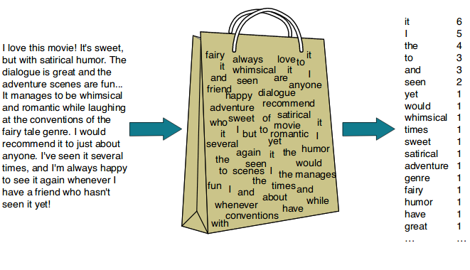
A bag-of-words model allows us to extract features from textual data. As we know, an algorithm doesn’t understand language. Thus, we need to use a numeric representation for the words in the corpus. This numeric representation can later be fed to any algorithm for further analysis.

It’s called “bag-of-words” because the order of the words or the structure of the sentence is lost in this model. Only the occurrence or presence of a word matters.

We can think of the model in such a way — we have a big bag, empty at the start, and a vocabulary or a corpus. We pick up words one by one and put them in the bag, adding to the frequency of their occurrence, and then select the most common words as features for passing through our algorithm of choice.

Thus, it promotes the view that similar documents consist of similar kinds of words.

Dataset

The dataset that we’re going to use in this article is an SMS spam collection dataset. It contains over 5500 messages in English, with each message in a column, with the corresponding column next to it specifying whether the text is ham or spam.

You can find the dataset here. The complete source code can be found in thisrepository.

Importing the dataset

To import the dataset into a Pandas dataframe, we use the couple of lines written below:

import pandas as pd
dataset = pd.read_csv('spam.csv', encoding='ISO-8859-1');

Here’s a glimpse of the dataset we are working on. We, later convert the labels into dummy variables.

Pre-requisites

1. NLTK for NLP-related tasks
2. NumPy and Pandas for mathematical operations
3. Scikit-learn for tokenization and tf-idf model
4. Matplotlib and Seaborn for visualisation tasks

Data Pre-processing

Removing Stopwords

Stopwords refer to the words in the statement which add no specific meaning to it. They often involve prepositions, helping verbs, and articles (i.e. in, the, an, is). Since these add no value to our model, we need to eradicate them.

nltk.download('stopwords')
from nltk.corpus import stopwords
stopwords.words('english')

Removing non-alphabetic characters

Since we use only words for text classification, we need to get rid of punctuation and numbers. For this, we use string matching or regex in Python. The below regex only preserves alphabetic words, discarding the rest.

text = re.sub('[^A-Za-z]', ' ', text)

Changing all to lower case

The model cannot distinguish between lowercase and uppercase, treating ‘Text’ and ‘text’ as different words. We certainly don’t want that; thus, we change the case of all words to lowercase for simplicity.

text = text.lower()

Spelling Corrections

Sometimes, people write abbreviations or misspell words by mistake. To correct these instances, we use the autocorrect package and its spell corrector.

from autocorrect import spell
text.append(spell(word))

Stemming and Lemmatization

Words like act, actor, and acting all are for of the same root word (act).same Stemming and lemmatization are techniques used to truncate words in order to to get the stem or the base word.

The difference between these is that after stemming, the stem may not be an actual word, whereas lemmatization always produces a real world, which results in better interpretation of the corpora by humans.

For example, studies could be stemmed as studi (not a word), but will be lemmatized as study (an existing word).

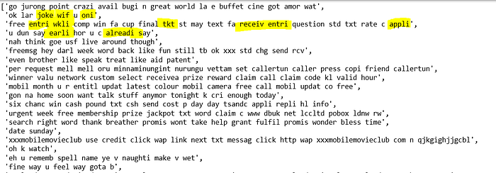
Here’s is a comparison of the dataset after and before stemming.

You can notice the highlighted words are among a few to be stemmed. Also, stemmed words are not actual words most of the time.

Visualizing Spam Keywords

Data visualization is a handy way of better understanding the text data involved in our dataset. For example, we can make a wordcloud, which represents most common words in a space, with the size of each word proportional to the frequency of its occurrence. A few other visualization techniques are discussed here.

from wordcloud import WordCloud
import matplotlib.pyplot as plt
spam_wc = WordCloud(width = 600,height = 512).generate(spam_words)
plt.figure(figsize = (12, 8), facecolor = 'k')
plt.imshow(spam_wc)
plt.show()

Feature Engineering

Now we need to perform manipulation on the cleaned, pre-processed dataset to transform it into a form more suitable for applying a machine learning algorithm.

Tokenisation

For the bag of words implementation, we use CountVectorizer from scikit-learn, which counts the frequency of each word present in our pre-processed dataset, and takes the n most common words as features.

CountVectorizer returns a matrix, where the rows contain the count of messages containing the word, and columns are the top selected features.

from sklearn.feature_extraction.text import CountVectorizer
data = CountVectorizer(max_features=2000)
X = data.fit_transform(dataset).toarray()

Since the countvectoriser contains 2000 features, they are hard to depict here. Thus, for an example below,we take the first 25 words of our dataset, tokenise them and select 10 of the most frequently used ones.

The matrix that represents the frequency of each of these features in our messages(dataset) is given below:

Developing the Model

Now that our dataset is ready with its attributes, we pass it through any algorithm of our choice. Here, after splitting the dataset into training and test sets, I’ve used a simple Naive Bayes classifier for demonstration. You can use any algorithm of your choice depending on the dataset.

from sklearn.model_selection import train_test_split
X_train, X_test, y_train, y_test = train_test_split(X, y)from sklearn.naive_bayes import GaussianNB
classifier = GaussianNB()
classifier.fit(X_train, y_train)
y_pred = classifier.predict(X_test)

Results

Let’s see how our simple model works on a test set:

Looks like our model crossed the finish line with a decent accuracy of ~80%. Not something to boast about, but still pretty decent given the simplicity of our model and its drawbacks, which are discussed in the next section. Thus, we can say that our model differentiates between ham and spam with a good confidence level.

Here is an image of the confusion matrix depicting the true positives and false positives in the first row and false negatives and true negatives in the next row respectively.

Drawbacks of the Bag-of-Words Model

The bag-of-words model assumes that the words are independent. Thus, it doesn’t take into account any relationship between words. Hence, the meaning of sentences is lost.

Also, the structure of the sentence has no importance in the eyes of our model Two sentences like “These clams are good” and “Are these clams good?” mean the same to the of bag-of-words model, though one is a claims and one is a question. Additionally, for a large vocabulary, bag-of-words result in a very high-dimensional vector.

Improvements to the above model

A few ways to improve the accuracy of the above model include:

1. Using custom-made stopwords, as per the dataset’s requirements(what language or lingo your dataset use), you can add other words according to the language of the corpus. Some of the text or links are specific to spam mails, or some lingo is added to pass generic spam filters. This can be avoided by analyzing the dataset well and knowing about the structure and content of spam messages specifically, tailoring stopwords to our needs.
2. Instead of using uni-grams (individual words), using bi-grams and tri-grams can be beneficial to better understand a message’s meaning. For example, take a message — “gift card worth millions”. Here, instead of using uni-grams, which would give us ‘gift’, ‘card’, ‘worth’, ‘millions’, we can use bi-grams that give us ‘gift card’ or ‘worth millions’ together as one feature. As you can see, this could clearly indicate a spam message, whereas ‘gift’, ‘card’, ‘worth’, and ‘millions’ could individually be a part of any day-to-day conversation.
3. Apply a vector space model like cosine similarity between messages, and use tf-idf vectorization to better understand the relative weight of a word to that document’s importance. You can read more about this here in this article.

Repository

Here’s the link to my repository, where you can find the complete source code for this tutorial. Also, I will keep on adding code on spam filtering using other techniques soon, so stay connected.

Sources to get started with NLP

Conclusion

In this post, we implemented a spam text classifier using a bag-of-words model. We learned how to work efficiently with text data and develop a reliable model using a few of NLP concepts.

There is a lot more to NLP, and spam filtering in general is a mature field, with various machine learning and deep learning techniques commonly used to improve model results. In future posts, I’ll try to approach spam filtering with different techniques. All feedback is welcome. Please help me improve!

Until next time!😁