Selecting the right weight initialization for your deep neural network

Part 1 of a two part series

The weight initialization technique you choose for your neural network can determine how quickly the network converges or whether it converges at all. Although the initial values of these weights are just one parameter among many to tune, they are incredibly important. Their distribution affects the gradients and, therefore, the effectiveness of training.

In neural networks, weights represent the strength of connections between units in adjacent network layers. The linear transformation of these weights and the values in the previous layer passes through a non-linear activation function to produce the values of the next layer. This process happens layer to layer during forward propagation; through back propagation, the optimum values of these weights can be found out so as to produce accurate outputs given an input.

In this article, we’ll cover:

• Why weight initialization is important
• Active areas of research around weight initialization

We will not be covering mathematical derivations of these initialization approaches. If you are interested in this type of material, we do link to several great resources within and at the end of the article (in the ‘Further Reading’ section) .

Why is weight initialization important?

Improperly initialized weights can negatively affect the training process by contributing to the vanishing or exploding gradient problem. With the vanishing gradient problem, the weight update is minor and results in slower convergence — this makes the optimization of the loss function slow and in a worst case scenario, may stop the network from converging altogether. Conversely, initializing with weights that are too large may result in exploding gradient values during forward propagation or back-propagation (see more here).

Deeplearning.ai recently published an interactive post where you can choose different initialization methods and watch the network train. Here’s an example:

You’ll notice how setting an initialization method that’s too small barely allows the network to learn (ie. reduce the cost function) while an initialization method that’s too large causes divergence (check the decision boundary).

How approaches for weight initialization have shifted?

In 2012, AlexNet, the winner of that year’s ImageNet Large Scale Visual Recognition Challenge (ILVSRC), popularized the weight initialization approach of “initialization with Gaussian (normal) noise with mean equal to zero and standard deviation set to 0.01 with bias equal to one for some layers” (see Krizhevsky et al. 2012).

However, this normal random initialization approach does not work for training very deep networks, especially those that use the ReLU (rectified linear unit) activation function, because of the vanishing and exploding gradient problem referenced earlier.

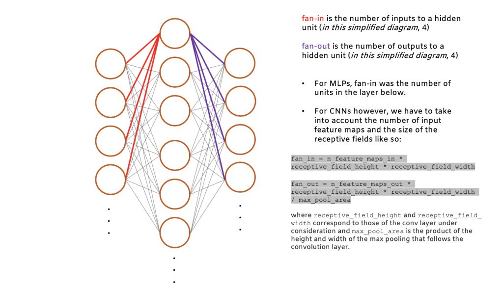
To address these issues, Xavier and Bengio (2010) proposed the “Xavier” initialization which considers the size of the network (number of input and output units) while initializing weights. This approach ensures that the weights stay within a reasonable range of values by making them inversely proportional to the square root of the number of units in the previous layer (referred to as fan-in). See the diagram below on how to find the fan-in and fan-out for a given unit:

The choice of activation function ends up playing an important role in determining how effective the initialization method is. Activation functions are differentiable and introduce non-linear properties (i.e. curvature) into our neural networks that are crucial for solving the complex tasks that machine learning and deep learning are designed to tackle.

The activation function is the non linear transformation that we do over the input signal. This transformed output is then sent to the next layer of units as input. Some examples of these non-linear activation functions are:

• Sigmoid
• Softmax
• Tanh
• ReLU
• Leaky ReLU

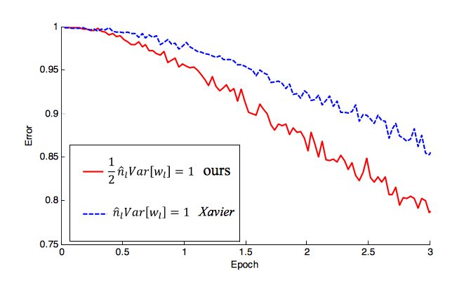
Rectified Linear unit (ReLU) (and leaky ReLU) are commonly used since they are relatively robust to the vanishing/exploding gradient issues. For activation functions like ReLU, Kaiming He et al. (2015) introduced a more robust weight initialization method that accounts for the fact that it’s not symmetric (see performance differenced cited in the He et al. paper below). Both methods use a similar theoretical analysis: they find a good variance for the distribution from which the initial parameters are drawn. This variance is adapted to the activation function used and is derived without explicitly considering the type of the distribution.

Figure from the He et al. (2015) paper showing how their refined initialization strategy (red) reduces the error rate much faster than the Xavier method (blue) for (P)ReLUs and accounts for the fact that it is not symmetric.

For an accessible proof of the Xavier and He initialization methods, see Pierre Ouannes’ excellent post ‘How to initialize deep neural networks? Xavier and Kaiming initialization’.

It’s important to note that weight initialization is still an active area of research. Several interesting research projects have popped up including data-dependent initializations, sparse weight matrices, and random orthogonal matrix initializations.

One of the most interesting developments in this area is MIT’s Lottery Ticket Hypothesis, which details how these large neural nets contain smaller “subnetworks” that are up to 10 times smaller than the full network. According to the research team, these subnetworks can learn just as well, making equally precise predictions sometimes faster than the full neural networks.

The authors of ‘The Lottery Ticket Hypothesis: Finding Sparse, Trainable Neural Networks’, Carbin and Frankle, tested their lottery ticket hypothesis and the existence of subnetworks by performing a process called pruning, which involves eliminating unneeded connections from trained networks based on their network prioritization or weight to fit them on low-power devices.

In fact, TensorFlow recently announced a new weight pruning API:

Weight pruning means eliminating unnecessary values in the weight tensors. We are practically setting the neural network parameters’ values to zero to remove what we estimate are unnecessary connections between the layers of a neural network. This is done during the training process to allow the neural network to adapt to the changes.

Read more about the weight pruning API here.

Interactive Demo

Try out this interactive demo here. The size of the weight values matter but making sure that the weights are randomly initialized is also critical. This random initialization approach is based off of a known property called Break Symmetry where:

• If two hidden units have the same inputs and same activation function, then they must have different initial parameters
• It’s desirable to initialize each unit to compute a different function

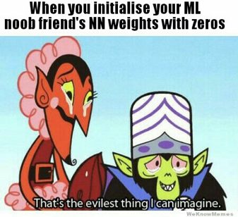
If the weights are initialized with just zeros, every neuron in the network would compute the same output, and gradients would undergo the exact same parameter updates. In other words, the units in the neural network will learn the same features during training if their weights are initialized to be the same value.

With transfer learning, instead of starting from randomly initialized weights, you use weights saved from a previous network as the initial weights for your new experiment (i.e. fine-tuning a pre-trained network).

Want to stay in the loop? Subscribe to the Comet Newsletter for weekly insights and perspective on the latest ML news, projects, and more.