Often in machine learning, and specifically with classification problems, we encounter imbalanced datasets. This typically refers to an issue where the classes are not represented equally, which can cause huge problems for some algorithms.

In this article, we’ll explore a technique called resampling, which is used to reduce this effect on our machine learning algorithms.

This article presumes that you know some machine learning concepts and are familiar with Python and its data science libraries.

What is an Imbalanced Dataset?

The best way to learn something is through an example:

Say that you have a fraud detection binary classification model (two classes — “Fraud” or “Not-Fraud”) problem with 100 instances (rows). A total of 80 instances are labeled as Fraud and the remaining 20 instances are labeled as a Not-Fraud. This is an imbalanced dataset, and the ratio of Fraud to Not-Fraud instances is 80:20, or 4:1.

Most classification datasets don’t have exactly equal numbers of records in each class, but a small difference doesn’t matter as much.

This class imbalance problem can occur in binary classification problems as well as multi-class classification problems, but most techniques can be used on either.

Project setup

In addition to using the core Python libraries like NumPy, Pandas, and scikit-learn, we’re going to use another great library called imbalanced-learn, which is a part of scikit-learn-contrib projects.

imbalanced-learn provides more advanced methods to handle imbalanced datasets like SMOTE and Tomek Links.

Here are the commands to install it via pip or conda:

# using pip
pip install -U imbalanced-learn# using conda
conda install -c conda-forge imbalanced-learn

The Metric Problem

Most beginners struggle when dealing with imbalanced datasets for the first time. They tend to use accuracy as a metric to evaluate their machine learning models. This intuitively makes sense, as classification accuracy is often the first measure we use when evaluating such models.

Nevertheless, this can be misleading, because most of the algorithms we use are designed to achieve the best accuracy, so the classifier always “predicts” the most common class without performing any features analysis. It will still have a high accuracy rate, but it will give false predictions, nevertheless.

Example

Say we have 1000 emails as a dataset: 990 are spam emails and 10 aren’t. If you build a simple model you’ll get ~99% accuracy, which at first glance seems great.

But on the other hand, the algorithm doesn’t perform any learning — the accuracy here is only reflecting the underlying class distribution because models look at the data and cleverly decide that the best thing to do is to always predict spam and achieve high accuracy. As such, the model’s success and is just an illusion.

This is why the choice of metrics used when working with imbalanced datasets is extremely important.

Investigate your dataset

You should have an imbalanced dataset to apply the methods described here— you can get started with this dataset from Kaggle.

You can use Seaborn to plot the count of each class to see if your dataset presents imbalanced dataset problem like the following:

# import the data sciecne libraries.
import pandas as pd
import matplotlib.pyplot as plt
import seaborn as sns

# read the dataset
data = pd.read_csv('training.csv')

# print the count of each class from the target vatiables
print(data.FraudResult.value_counts())

# plot the count of each class from the target vatiables
sns.countplot(data.FraudResult)

Or you can use the sklearn to compute class weight and get the class ratios as follows:

# import the function to compute the class weights
from sklearn.utils import compute_class_weight

# calculate the class weight by providing the 'balanced' parameter.
class_weight = compute_class_weight('balanced', data.FraudResult.unique() , data.FraudResult)

# print the result
print(class_weight)

Join more than 14,000 of your fellow machine learners and data scientists. Subscribe to the premier newsletter for all things deep learning.

Resampling

There are multiple ways to handle the issue of imbalanced datasets. The techniques we’re going to use in this tutorials is called resampling.

Resampling is a widely-adopted technique for dealing with imbalanced datasets, and it is often very easy to implement, fast to run, and an excellent starting point.

Resampling changes the dataset into a more balanced one by adding instances to the minority class or deleting ones from the majority class, that way we build better machine learning models.

The way to introduce these changes in a given dataset is achieved via two main methods: Oversampling and Undersampling.

• Oversampling: This method adds copies of instances from the under-represented class (minority class) to obtain a balanced dataset. There are multiple ways you can oversample a dataset, like random oversampling. We’ll cover some of these methods in this article.

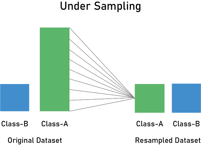
• Undersampling methods: These methods simply delete instances from the over-represented class (majority class) in different ways. The most obvious way is to do delete instances randomly.

Disadvantages

Notwithstanding the advantage of balancing classes, these techniques also have some drawbacks:

• If you duplicate random records from the minority class to do oversampling, this will cause overfitting.
• By undersampling and removing random records from the majority class, you risk losing some important information for the machine learning algorithm to use while training and predicting.

We’ll now show the underlying techniques in each method, along with some code snippets.

Undersampling

Random Undersampling

Random undersampling randomly deletes records from the majority class. You should consider trying this technique when you have a lot of data.

A simple undersampling technique is to undersample the majority class randomly and uniformly. This can potentially lead to information loss, though. But if the examples of the majority class are near to others in terms of distance, this method might yield good results.

Here is a code snippet:

# import the Random Under Sampler object.
from imblearn.under_sampling import RandomUnderSampler

# create the object.
under_sampler = RandomUnderSampler()

# fit the object to the training data.
x_train_under, y_train_under = under_sampler.fit_sample(x_train, y_train)

Here’s the set of parameters you can specify to the RandomUnderSampler object (the same thing apply for the other objects from the imblearn library):

• sampling_strategy : This parameter can be used to tell the object how to perform undersampling on our dataset. It can be majority to resample only the majority class, not_minority to resample all classes but the minority class, and auto is the default one here, which stands for not_minority. You can check out the documentation (included below in “Resources”) to learn more.
• return_indices : Boolean on whether to return the indices of the removed instances or not.
• random_state : An integer that controls the randomness of the procedure, allowing you to reproduce the results.

NearMiss Undersampling

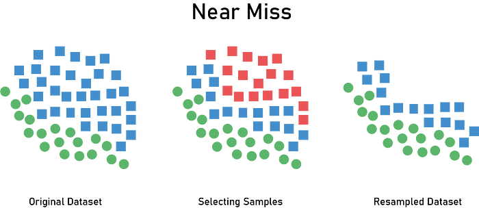
The NearMiss algorithm has been proposed to solve the issue of potential information loss. It’s based on the nearest neighbor algorithm and has a lot of variations that we’ll see in this section.

The basics of the NearMiss algorithms include the following:

1. The method starts by calculating the distances between all instances of the majority class and the instances of the minority class.
2. Then k instances of the majority class that have the smallest distances to those in the minority class are selected to be retained.
3. If there are n instances in the minority class, NearMiss will result in k × ninstances of the majority class.

Here are the different versions of this algorithm:

• NearMiss-1 chooses instances of the majority class where their average distances to the three closest instances of the minority class are the smallest.
• NearMiss-2 uses the three farthest samples of the minority class.
• NearMiss-3 picks a given number of the closest samples of the majority class for each sample of the minority class.

Here is a code snippet:

# import the NearMiss object.
from imblearn.under_sampling import NearMiss

# create the object with auto
near = NearMiss(sampling_strategy="not minority")

# fit the object to the training data.
x_train_near, y_train_near = near.fit_sample(x_train, y_train)

You can tune also the following parameters:

• version : the version of the near-miss algorithm, which can be 3,1, or 2.
• n_neighbors : the number of neighbors to consider to compute the average distance—three is the default.

Undersampling with Tomek links

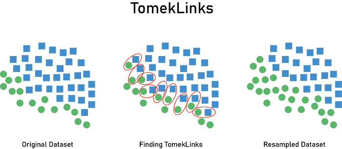
Tomek links are pairs of very close instances that belong to different classes. They’re samples near the borderline between classes. By removing the examples of the majority class of each pair, we increase the space between the two classes and move toward balancing the dataset by deleting those points.

Here is a code snippet to resample the majority class:

# import the TomekLinks object.
from imblearn.under_sampling import TomekLinks

# instantiate the object with the right ratio strategy.
tomek_links = TomekLinks(sampling_strategy='majority')

# fit the object to the training data.
x_train_tl, y_train_tl = tomek_links.fit_sample(x_train, y_train)

Undersampling with Cluster Centroids

The idea here is basically to remove the unimportant instance from the majority class. To decide whether an instance is important or not, we use the concept of clustering on the geometry of the feature space.

Clustering is an unsupervised learning approach, in which clusters are creating encircling data points belonging.

We will use it only to find cluster centroid that are obtained by averaging feature vector for all the features over the data points.

After finding the cluster centroid of the majority class, we decide the following:

• The instance belonging to the cluster (majority class), which is farthest from the cluster centroid in the feature space, is considered to be the most unimportant instance.
• The instance belonging to the majority class, which is nearest to the cluster centroid in the feature space, is considered to be the most important instance.

Here is a code snippet for using cluster centroids:

# import the ClusterCentroids object.
from imblearn.under_sampling import ClusterCentroids

# instantiate the object with the right ratio.
cluster_centroids = ClusterCentroids(sampling_strategy="auto")

# fit the object to the training data.
x_train_cc, y_train_cc = cluster_centroids.fit_sample(x_train, y_train)

Besides the previous parameter, here’s another one you can tune to get better results:

• estimator: An object that performs the clustering process for this method—K-Means is the default here.

Undersampling with Edited Nearest Neighbor Rule

Edited Nearest Neighbor Rule (or ENN) was proposed in 1972 to remove instances from the majority class (undersampling).

This technique removes any instance from the majority class whose class label is different from the class label of at least two of its three nearest neighbors. In general terms, it’s near or around the borderline of different classes.

The point here is to increase the classification accuracy of minority instances rather than majority instances.

Here is a sample code snippet:

# import the EditedNearestNeighbours object.
from imblearn.under_sampling import EditedNearestNeighbours

# create the object to resample the majority class.
enn = EditedNearestNeighbours(sampling_strategy="majority")

# fit the object to the training data.
x_train_enn, y_train_enn = enn.fit_sample(x_train, y_train)

Undersampling with Neighborhood Cleaning Rule

Neighborhood Cleaning Rule ( or NCR) deals with the majority and minority samples separately when sampling the datasets.

NCR starts by calculating the nearest three neighbors for all instances in the training set. We then do the following:

• If the instance belongs to the majority class and the classification given by its three nearest neighbors is the opposite of the class of the chosen instance — then the chosen instance is removed.
• If the instance belongs to the minority class and it’s misclassified by its three nearest neighbors — then the nearest neighbors that belong to the majority class are removed.

Here is a sample code snippet:

# import the NeighbourhoodCleaningRule object.
from imblearn.under_sampling import NeighbourhoodCleaningRule

# create the object to resample the majority class.
ncr = NeighbourhoodCleaningRule(sampling_strategy="majority")

# fit the object to the training data.
x_train_ncr, y_train_ncr = ncr.fit_sample(x_train, y_train)

An important parameter here is threshold_clearning, which is a float number used after applying ENN, it tells the algorithm to consider a class or not during the cleaning.

Oversampling

Random Oversampling

Random oversampling randomly duplicate records from the minority class. Try this technique when you don’t have a lot of data.

Random oversampling simply replicates random minority class examples. It’s known to increase the likelihood of overfitting, which is a major drawback.

Here is a sample code snippet:

# import the Random Over Sampler object.
from imblearn.over_sampling import RandomOverSampler

# create the object.
over_sampler = RandomOverSampler()

# fit the object to the training data.
x_train_over, y_train_over = over_sampler.fit_sample(x_train, y_train)

SMOTE Oversampling

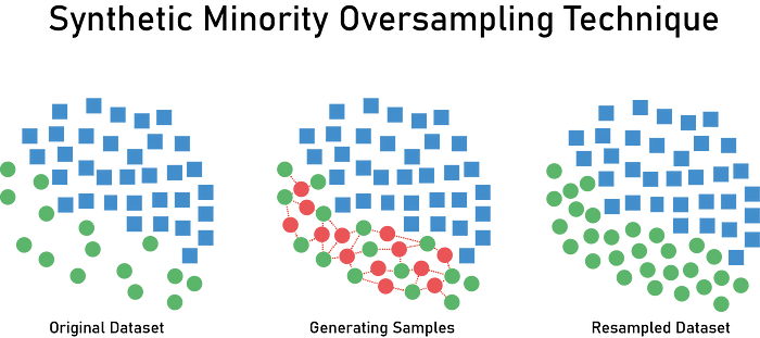
SMOTE stands for Synthetic Minority Oversampling Technique — it consists of creating or synthesizing elements or samples from the minority class rather than creating copies based on those that exist already. This is used to avoid model overfitting.

To create a synthetic instance, SMOTE finds the K-nearest neighbors of each minority instance, randomly selects one of them and then calculates linear interpolations to produce a new minority instance in the neighborhood. It can be also explained by changing this instance features one at a time by a random amount — so as a result, the new points are added between the neighbors.

Here is a code snippet showing how to resample the minority class:

# import the SMOTETomek
from imblearn.over_sampling import SMOTE

# create the  object with the desired sampling strategy.
smote = SMOTE(sampling_strategy='minority')

# fit the object to our training data
x_train_smote, y_train_smote = smote.fit_sample(x_train, y_train)

ADASYN Oversampling

ADASYN stands for Adaptive Synthetic sampling, and as SMOTE does, ADASYN generates samples of the minority class. But here, because of their density distributions, this technique receives wide attention.

Its purpose is to generate data for minority class samples that are harder to learn, as compared to those minority samples that are easier to learn.

It measures the K-nearest neighbors for all minority instances, then calculates the class ratio of the minority and majority instances to create new samples.

Repeating this process, we will adaptively shift the decision boundary to focus on those samples that are hard to learn.

Here is a code snippet:

# import the ADASYN object.
from imblearn.over_sampling import ADASYN

# create the object to resample the majority class.
adasyn = ADASYN(sampling_strategy="minority")

# fit the object to the training data.
x_train_adasyn, y_train_adasyn = adasyn.fit_sample(x_train, y_train)

Combining Oversampling and Undersampling

We can combine oversampling and undersampling techniques to get better sampling results. Here are two ways that imblearn provides:

SMOTE & Tomek Links — Here’s a code snippet:

# import the SMOTETomek.
from imblearn.combine import SMOTETomek

# create the  object with the desired sampling strategy.
smotemek = SMOTETomek(sampling_strategy='auto')

# fit the object to our training data.
x_train_smt, y_train_smt = smotemek.fit_sample(x_train, y_train)

SMOTE & Edited Nearest Neighbor — Here’s a code snippet:

# import the SMOTEENN.
from imblearn.combine import SMOTEENN

# create the  object with the desired samplig strategy.
smoenn = SMOTEENN(sampling_strategy='minority')

# fit the object to our training data.
x_train_smtenn, y_train_smtenn = smoenn.fit_sample(x_train, y_train)

Other Techniques

Besides the resampling methodologies we’ve covered in this article, there are other intuitive and advanced techniques you can employ to deal with this problem. Here are some of them:

1. Collect more data: You can always collect more data from other sources to build a more robust model.
2. Changing the performance metric: We’ve seen that accuracy is misleading — it’s not the metric to use when dealing with imbalanced datasets. Some metrics have been designed for such a case, including: Confusion Matrix, Precision & Recall, F1 Score, ROC Curves.
3. Use different algorithms: Some algorithms are better than others when dealing with imbalanced datasets. Generally, in machine learning, we test a variety of different types of algorithms on a given problem to see which ones provide better performance.
4. Use penalized models: Some algorithms allow you to give them a different perspective on the problem. For instance, with some algorithms, we can add costs to force the model to pay attention to the minority class. There are penalized versions of algorithms such as penalized-SVM and logistic regression, even when using deep learning models throughout the class_weight attribute.

Resources

There are more resources out there to handle your imbalanced dataset. Here are a few to help you get started:

• How to set class weights for the imbalanced dataset in Keras
• The imbalanced-learn documentation.
• Another undersampling method called Condensed Nearest Neighbour.

Conclusion

In this article, we confronted the problem of imbalanced datasets by exploring several different resampling techniques, which allow you to change your dataset’s balance so your model can learn more effectively.

You’ll need to experiment with these techniques on your specific machine learning problem to see what best fits your case — we don’t have a technique that always allows us to build a better model while achieving the best performance. Otherwise, we wouldn’t be able to say that we’re machine learning engineers.

You can combine these methods to obtain more reliable models, but I suggest starting small and building upon what you learn.