Running deep learning models is computationally expensive. And when it comes to image processing with computer vision, the first thing that comes to mind is high-end GPUs—think the 1080ti and now the 2080ti.

But it’s hard to run computer vision models on edge devices like Raspberry Pi, and making a portable solution is difficult with deep learning libraries like TensorFlow or PyTorch.

For this task, it’s almost compulsory to add OpenCV to help pre-process data. And the good news is that OpenCV itself includes a deep neural network module, known as OpenCV DNN. It runs much faster than other libraries, and conveniently, it only needs OpenCV in the environment. As a result, OpenCV DNN can run on a CPU’s computational power with great speed.

The best use case of OpenCV DNN is performing real-time object detection on a Raspberry Pi. This process can run in any environment where OpenCV can be installed and doesn’t depend on the hassle of installing deep learning libraries with GPU support. As such, this tutorial isn’t centered on Raspberry Pi—you can follow this process for any environment with OpenCV.

How Does Object Detection with OpenCV DNN Work?

Previously, I wrote this piece:

Without TensorFlow: Web app with an Object Detection API in Heroku and OpenCV [LINK]

While writing the above article, I realized there are lots of code examples available online, but I couldn’t find any output analysis using OpenCV DNN for object detection. So I figured, why not explore the OpenCV DNN module?

So in this tutorial, we’ll be exploring how object detection works with OpenCV DNN and MobileNet-SSD (in terms of inference).

We’ll be using:

1. Python 3
2. OpenCV [Latest version]
3. MobileNet-SSD v2

OpenCV DNN supports models trained from various frameworks like Caffe and TensorFlow. It also supports various networks architectures based on YOLO, MobileNet-SSD, Inception-SSD, Faster-RCNN Inception,Faster-RCNN ResNet, and Mask-RCNN Inception.

Because OpenCV supports multiple platforms (Android, Raspberry Pi) and languages (C++, Python, and Java), we can use this module for development on many different devices.

Why OpenCV DNN?

OpenCV DNN runs faster inference than the TensorFlow object detection API with higher speed and low computational power. We will see the performance comparison in a future blog post.

Why MobileNet-SSD?

MobileNet-SSD can easily be trained with the TensorFlow-Object-Detection-API, Lightweight.

Check out the official docs for more.

Getting Started

First things first, here’s a GitHub repo I created that allows you to explore this module:

Installation

Installing OpenCV for python

pip3 install opencv-python

Download the pre-trained model from the above link.

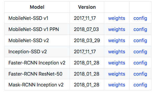
We’ll be using MobileNet-SSD v2 for our object detection model, as it’s more popular—let’s download its weights and config.

From the weights folder (after unzipping), we use the frozen_inference_graph.pb file.

Project Structure

(I’m using virtualenv for this tutorial, so there is venv, but this isn’t mandatory.)

Lets code

All of the code can be found in main.py

classNames is a dictionary that contains the 90 objects trained in the model and also in the background 

Loading models (Those we have downloaded)

model = cv2.dnn.readNetFromTensorflow('models/frozen_inference_graph.pb', 'models/ssd_mobilenet_v2_coco_2018_03_29.pbtxt')

We need an image to detect objects (these can be captured as frames from live video)

For the purposes of this tutorial, let’s use this image:

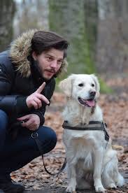
Download the image into the code directory; then read the image with OpenCV and show it:

image = cv2.imread("image.jpeg")
cv2.imshow('image',image)
cv2.waitKey(0)
cv2.destroyAllWindows()

Feeding the image to the network

To feed image into the network, we have to convert the image to a blob. A blob is a pre-processed image that serves as the input. Pre-processing techniques like resizing according to the model, color swapping, cropping, and color channels mean subtraction (normalizing color channel values by subtracting a mean value).

model.setInput(cv2.dnn.blobFromImage(image, size=(300, 300), swapRB=True))

We’re resizing the image to 300 x 300 as our pre-trained model supports and swapping the color channels from BGR to RGB. OpenCV reads in BGR, while RGB is commonly used in model training. RGB is more popular.

Feeding forward the model

output = model.forward()

We got the output, so now we need to understand it. For the input image we have given, the shape of the output matrix is (1, 1, 100, 7), Our main concern is output [0,0,:,:]

output[0,0,:,:].shape is (100, 7)

Thresholding Results

for detection in output[0,0,:,:]:
    confidence = detection[2]

Each detection output gives a predicted confidence in a range of 0 to 1. But most of them are false positive (falsely detected). So we’ll keep only objects of higher confidence. For that, let’s set a threshold of .5. We’ll consider everything up to that threshold when drawing the bounding box around the image.

if confidence > .5:

For the predicted class, we get the id. From the id, we’ll get the class name from the classNames dictionary.

class_id = detection[1]

Converting id to class name

This function below takes class_id and returns the class name according to the id from classNames

def id_class_name(class_id, classes):
    for key,value in classes.items():
        if class_id == key:
            return value

In this loop, we’re printing Class id, confidence, and class name for debugging purposes before drawing the box.

for detection in output[0, 0, :, :]:
    confidence = detection[2]
    if confidence > .5:
        class_id = detection[1]
        print(str(str(class_id) + " " + str(detection[2])  + " " + id_class_name(class_id,classNames)))

This is the output we got from the above code:

1.0 0.6377985 person
18.0 0.84042233 dog

The Bounding Box

It’s time to draw the box in the image. To draw the bounding box in the image for the predicted object, we need x, y, width, and height.

box_x=detection[3]
box_y=detection[4]
box_width=detection[5]
box_height=detection[6]

But we need to scale the values of the box according to our image height and width. But the image is 3 dimensional, as it also includes color channels, and we’re only taking height and width. So we skip the color channel input with “_”

image_height, image_width, _ = image.shape

After scaling

box_x = detection[3] * image_width
box_y = detection[4] * image_height
box_width = detection[5] * image_width
box_height = detection[6] * image_height

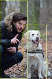
Once we’ve scaled the image, we have to draw the box with those new values in the image

cv2.rectangle(image, (int(box_x), int(box_y)), (int(box_width), int(box_height)), (23, 230, 210), thickness=1)

OpenCV’s rectangle function takes arguments for the image input, rectangle x, rectangle y, rectangle width, and rectangle height. It also takes color and thickness.

Adding Text

Now that we’ve drawn the bounding boxes, let’s add the class text in the box:

cv2.putText(image,class_name ,(int(box_x), int(box_y+.05*image_height)),cv2.FONT_HERSHEY_SIMPLEX,(.005*image_width),(0, 0, 255))

OpenCV’s putText function takes arguments for image, text, starting x, starting y, font type, font size, and text color. In the above code snippet, We’ve scaled the starting y and font size according to the image dimensions.

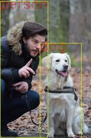
Voilà! Now we’ve got our desired bounding box in the detected objects, and we’ve added labels to each of them.

Conclusion

My hope is that this tutorial has provided an understanding of how we can use the OpenCV DNN module for object detection. And with MobileNet-SSD inference, we can use it for any kind of object detection use case or application.

Now that we have an understanding of the output matrix, we can use the output values according to our application’s need. It gets more fun when you run a custom-trained model—maybe we can see this in a future blog post!

Discuss this post on Hacker News and Reddit.

Find me:

GitHub: https://github.com/rdeepc

LinkedIn: https://www.linkedin.com/in/saumyashovanroy/