Pythae + Comet
The Pythae library, which brings together many Variational Autoencoder models and enables researchers to make comparisons and conduct reproducible research, is now integrated with Comet ML!
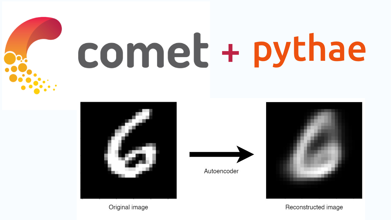
The Comet ML experiment tracking tool is very useful for researchers to store their experiment configs, track their training, and compare the results in an easy and understandable way through a visual interface.
Now let’s see in practice how to easily monitor an experiment with Comet ML in Pythae!
What is a (Variational) Autoencoder?
Images, texts, sounds, and more, produced realistically with deep neural networks, have come to the fore in recent years as the output of surprisingly talented models.
Although these generative models, which are well-designed and require huge data, appear in the literature with many different architectures, the Generative Attractive Networks and Variable Autoencoders model families are at the forefront of this race!
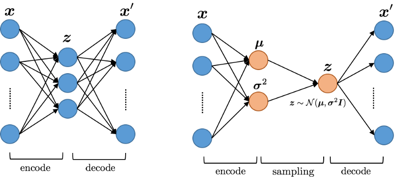
Autoencoders are non-generative models that aim to automatically learn to convert any data to code, consisting of two basic parts, an Encoder and a Decoder. Its main purpose is to compress the data given as input and reproduce it with as little loss as possible. The Variational Autoencoder family, on the other hand, includes generator models that have the ability to generate random codes by sampling and obtain new data with this code.

The idea of Variational Autoencoder was presented in 2013 by Diederik P. Kingma and Max Welling in the article “Auto-Encoding Variational Bayes.”
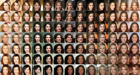
What distinguishes the models in this family from standard Autoencoders is that the input passed through the Encoder is encoded as a probability distribution. If this probability distribution is, for example, a normal distribution, the Encoder output will be the mean and variance values. By sampling these values, the code is obtained and this code can be solved with the help of a Decoder. Although the Decoder structure is the same in Standard and Variational Autoencoder models, there is a difference in the Encoder structure.
With Auto Encoder, they can be trained easily with a single loss function without the need for extra parameters. In Variational Encoders, on the other hand, it is difficult and challenging to find the balance between reconstruction and latent loss, so training is quite difficult. However, the fact that Auto Encoders are prone to overfitting causes Variational Auto Encoders to be preferred.
What is Pythae?
Pythae is a Python library that gathers the most commonly used (Variational) Auto-Encoder models under one roof, providing easy benchmarking experiments and comparison opportunities, especially for researchers.
It allows researchers to train any of the models it contains with their own data and allows the sharing and uploading of existing models on HuggingFace Hub. On the other hand, thanks to its integration with tools such as Comet, it allows you to monitor the experiments.
🟠 You can install the latest stable version of the pythae library using pip: pip install pythae
🟠To install the latest version of the Pythae library: pip install git+https://github.com/clementchadebec/benchmark_VAE.git
Some models in the Pythae library: Autoencoder (AE), Variational Autoencoder (VAE), Beta Variational Autoencoder (BetaVAE), VAE with Linear Normalizing Flows (VAE_LinNF), VAE with Inverse Autoregressive Flows (VAE_IAF), Disentangled Beta Variational Autoencoder (DisentangledBetaVAE), Disentangling by Factorising (FactorVAE), Beta-TC-VAE (BetaTCVAE).
Some samplers available with the Pythae library: Normal prior (NormalSampler), Gaussian mixture (GaussianMixtureSampler), Two stage VAE sampler (TwoStageVAESampler), Unit sphere uniform sampler (HypersphereUniformSampler), Poincaré Disk sampler (PoincareDiskSampler), VAMP prior sampler (VAMPSampler).
You can find the complete list of models and samplers and all sample source codes for the library here.
What is Comet?
Comet is a platform that enables teams and individuals to manage key machine learning lifecycle steps such as monitoring, versioning, model registration, and comparing results, especially iterative model training processes performed by teams of data science and machine learning researchers. And now Comet is fully integrated with Pythae!
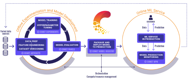
The Comet platform supports every stage of the machine learning lifecycle, from monitoring training runs to monitoring models in production. In addition, due to its flexible nature, it can be run with dozens of installation options both for the company and on any infrastructure, including virtual private cloud (VPC) installations. On the other hand, you can launch Comet easily and quickly by adding just two lines of code to your script, notebook, or pipeline. This will ensure that everything you need to monitor and manage your code, metrics and hyperparameters will be transferred to the platform.
Comet is free for individuals and you can create your account here.
The easiest way to install Comet on your system is to use pip: pip install comet_ml
Pythae + Comet
Now that we have an idea about Pythae and Comet, it’s time to practice!
The Variational Autoencoder (VAE) model has been implemented in the Pythae library. We will also train the reconstruction example in the MNIST dataset using the Pythae library and see how we can follow the training logs via Comet ML.
Importing Libraries
In PyTorch, you can import the torchvision package to use the vision datasets, the pythae package to train the reconstruction model practically, the CometCallback function of Pythae to monitor the logs, which includes the integration of Pythae and CometML, and the comet_ml package if you want to show the Comet UI directly in the Jupyter notebook.
import torchvision.datasets as datasets

#pythae
from pythae.models import BetaVAE, BetaVAEConfig
from pythae.trainers import BaseTrainerConfig
from pythae.pipelines.training import TrainingPipeline
from pythae.models.nn.benchmarks.mnist import Encoder_ResNet_VAE_MNIST, Decoder_ResNet_AE_MNIST

# Create you callback
from pythae.trainers.training_callbacks import CometCallback

# Or you can alternatively ability to view the Comet UI in the jupyter notebook
import comet_ml
Downloading the Dataset
Let’s download the MNIST dataset with the torchvision.datasets package. Then, let’s reshape it according to the input shape of the model by separating it as train and eval. Finally, let’s normalize.
mnist_trainset = datasets.MNIST(root='../data', train=True, download=True, transform=None)

train_dataset = mnist_trainset.data[:-10000].reshape(-1, 1, 28, 28) / 255.
eval_dataset = mnist_trainset.data[-10000:].reshape(-1, 1, 28, 28) / 255.
Defining Model Parameters
- Let’s define Trainer arguments:
training_config = BaseTrainerConfig(
    output_dir='my_model',
    learning_rate=1e-4,
    batch_size=100,
    num_epochs=10, # Change this to train the model a bit more,
    steps_predict=3
)
- Let’s define the VAE model arguments:
model_config = BetaVAEConfig(
    input_dim=(1, 28, 28),
    latent_dim=16,
    beta=2.

)
- To create the VAE model, let’s define the above config and Autoencoder’s encoder and decoder neural network model structure:
model = BetaVAE(
    model_config=model_config,
    encoder=Encoder_ResNet_VAE_MNIST(model_config),
    decoder=Decoder_ResNet_AE_MNIST(model_config)
)
Comet ML — Defining Callback
Before starting the training pipeline, we need to create the CometCallback. To access this feature;
- You must create a comet_ml account.
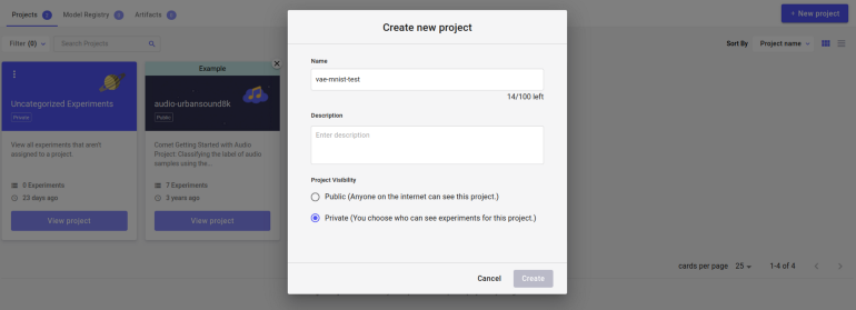
- You should create a new project under your account and note the project name.
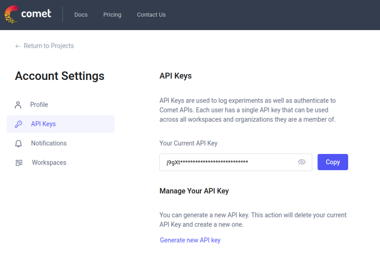
- You should create and note the API KEY from your Comet ML account settings.
- You can note down your Comet ML username as the default workspace name.
In order to be able to monitor on Comet ML, let’s define all the information we noted in the Comet setup arguments as follows and add it to the callbacks array upon adding it to the TrainingPipeline.
callbacks = [] # the TrainingPipeline expects a list of callbacks

comet_cb = CometCallback() # Build the callback

# SetUp the callback
comet_cb.setup(
    training_config=training_config, # training config
    model_config=model_config, # model config
    api_key={{API KEY}}, # specify your comet api-key
    project_name={{PROJECT NAME}}, # specify your wandb project
    workspace={{WORKSPACE NAME}}, #default workspace name = comet ml username
    #offline_run=True, # run in offline mode
    #offline_directory='my_offline_runs' # set the directory to store the offline runs
)

callbacks.append(comet_cb) # Add it to the callbacks list
As a result of these definitions, you will get a link output in the format `https://www.comet.com/{username}/{project_name}/{id}` to view the test results.
Training Pipeline Definition and VAE Training
Let’s define a training pipeline with the TrainingPipeline function of Pythae, the BaseTrainerConfig variable containing the model arguments we defined earlier, and the BetaVAE variable containing the VAE Autoencoder model structure.
pipeline = TrainingPipeline(
    training_config=training_config,
    model=model
)
Let’s start the training by giving the training and validation dataset and the callbacks array containing the CometCallback to the parameters of the pipeline we have defined as follows:
pipeline(
    train_data=train_dataset,
    eval_data=eval_dataset,
    callbacks=callbacks # pass the callbacks to the TrainingPipeline and you are done!
)
# You can log to https://comet.com/your_comet_username/your_comet_project to monitor your training
The training has started and the test results will immediately start to be displayed in the project you created in Comet ML.
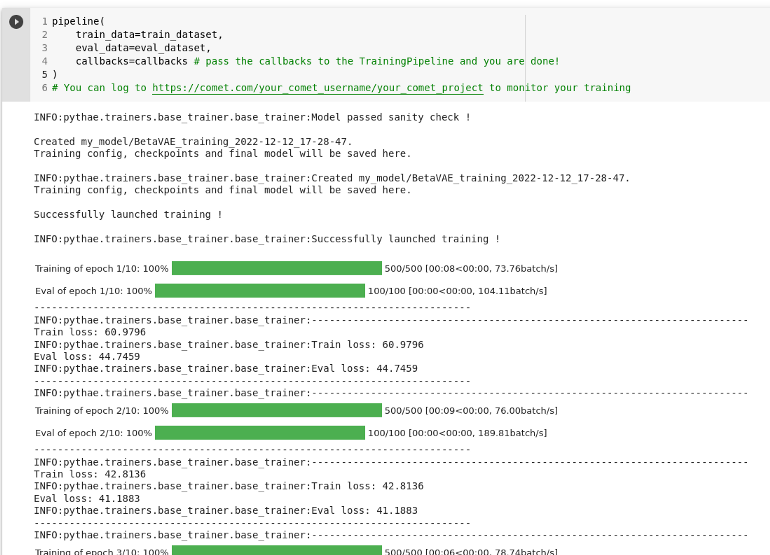
Train loss and eval loss graphs of the training can be viewed in real time via Comet ML.
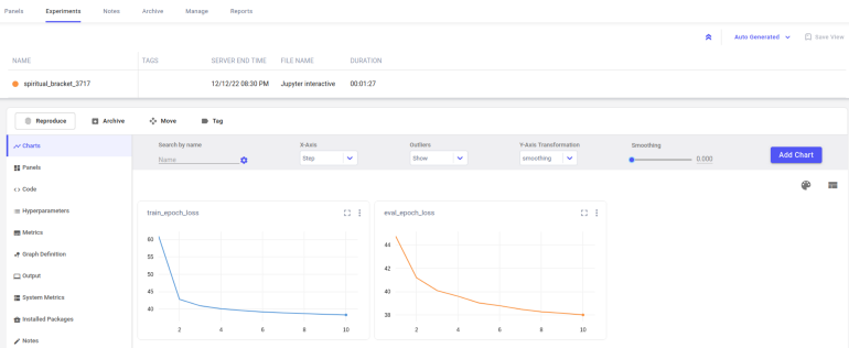
If you want to display the test results as Comet UI directly in a Jupyter Notebook, you can pull the test results with the `get_global_experiment()` function in the comet_ml package and display them with the `display()` function.
experiment = comet_ml.get_global_experiment()
experiment.display()
Other Features of Comet
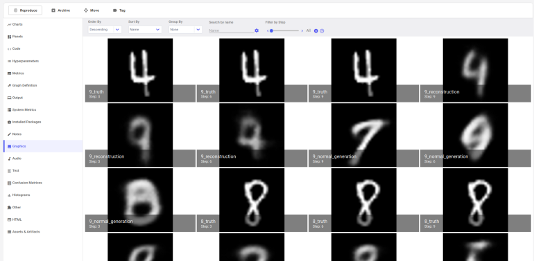
You can view the step by step outputs of the model in the Graphics page in the Experiment tab of Comet ML.
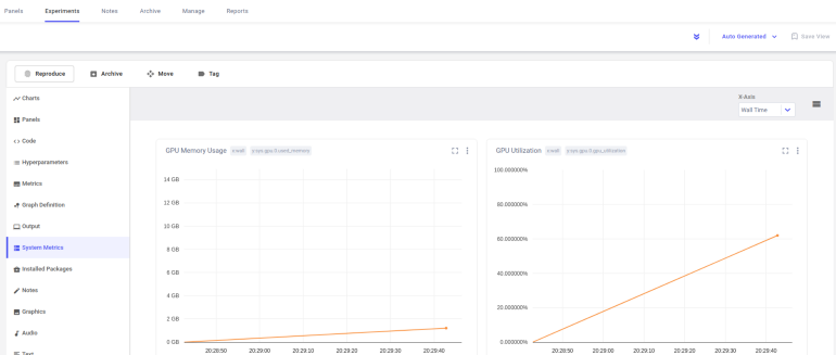
On the System Metrics page, you can see GPU Memory usage, CPU usage, and Memory usage values.
Conclusion
In this article we learned how you can follow the training logs of the model we used to reconstruct the images in the MNIST dataset and more by using the Comet ML tool, which is fully integrated with Pythae. Hope it was helpful!
References:

