Text-to-image generators are currently a red hot topic in the field of AI art. With them, a user can provide text describing the artwork they’d like to output, and the machine generates different variations of this image (sometimes in less than a minute!). Deep learning powers this technology, which helps anyone without design skills create artwork with just their sheer imagination. These AI systems have been trained using millions of images, along with their captions.

Some companies have trained their own AI “artists” and made them publicly available for people to use. Examples of such products include:

• DALL-E 2 by OpenAI is an AI system that pioneered this field. It is currently in public closed beta and you need to purchase credits to use it.
• Midjourney is an independent research lab that offers an AI program that creates images using textual descriptions. It is integrated with discord via a bot.
• Stable diffusion is a latent text-to-image diffusion model capable of generating photo-realistic images, given any text input. Created by Stability AI, they open-sourced a GitHub repository that has pre-trained models.

The main work involved in using these AI systems is coming up with textual descriptions of visuals you’d like to create. These descriptions, called “prompts,” can be as vague or as detailed as you’d like. The more specific your prompt is, the higher the level of fidelity of the image generated. The use of specific keywords can help to boost the quality of your image. For your reference, check out the Dalle-2 Prompt Book to get started with creating quality prompts.

In this article, you are going to analyze a dataset of 200K+ prompts created by Midjourney users. This dataset is available in HuggingFace and you are going to use it to:

• Create and visualize word embeddings;
• Perform a semantic search that will help you find similar prompts;
• Explore topics using clustering algorithms and visualize the keywords in each cluster.

Prerequisites

You will need to have python 3.6+ installed in your development environment in order to follow along with this hands-on tutorial. In addition, you need to create an account for Cohere.

Cohere is a platform that provides access to advanced large language models and NLP tools through one easy-to-use API. The platform offers free credits that you can use to experiment with your NLP projects.

Install the following python modules before getting started

pip install datasets cohere altair numpy pandas sklearn wordcloud matplotlib

Data preparation

The dataset is available on HuggingFace. You’ll need to download it, convert it to a pandas DataFrame, and finally, remove any empty strings:

from datasets import load_dataset
import pandas as pd
import numpy as npdataset = load_dataset(“succinctly/midjourney-prompts”)
df = dataset[‘test’].to_pandas()
df = df[df[‘text’].str.strip().astype(bool)]

Create and visualize word embeddings

Word embeddings are a way to represent text where words that have the same meaning have a similar representation. This representation helps machines understand languages and can be applied to natural language processing pipelines. For our use case, we’ll use word embeddings to explore similar prompts and cluster prompts into topics in an unsupervised manner.

To get started, you need to get your API key from Cohere’s platform. Log in to your account and create a key in the dashboard section as shown below:

Initialize the cohere plugin with your key and call the embed endpoint. The endpoint accepts a list of texts you want to process and returns a list of floating point numbers. Append the embeddings to the original DataFrame. You can learn more about Cohere’s Embed Endpoint here.

import cohere
co = cohere.Client('<api_key>')
df['text_embeds']=co.embed(model='small', 
                           texts=df['text'].tolist()).embeddings

To visualize the embeddings, you need to reduce them to two dimensions using Principal Component Analysis (PCA). Create two functions — one for creating the principal component analysis, and the other one for plotting a scatter plot:

from sklearn.decomposition import PCA
import altair as alt

# Compute the principal components
def get_pc(arr,n):
  pca = PCA(n_components=n)
  embeds_transform = pca.fit_transform(arr)
  return embeds_transform

# Generate scatter plots
def scatter_plot(df,xcol,ycol,color='basic',title=''):
  chart = alt.Chart(df).mark_circle(size=500).encode(
    x= alt.X(xcol,
      scale=alt.Scale(zero=False),
      axis=alt.Axis(labels=False, ticks=False, domain=False)
    ),
    y= alt.Y(ycol,
      scale=alt.Scale(zero=False),
      axis=alt.Axis(labels=False, ticks=False, domain=False)
    ),
    color= alt.value('#333293') if color == 'basic' else color,
    tooltip=['text']
  )
  result = chart.configure(background="#FFF"
        ).properties(
        width=800,
        height=500,
        title=title
       ).configure_legend(
  orient='bottom', titleFontSize=18,labelFontSize=18)
  return result

With the two functions created, calculate the principal components using the word embeddings, then plot them:

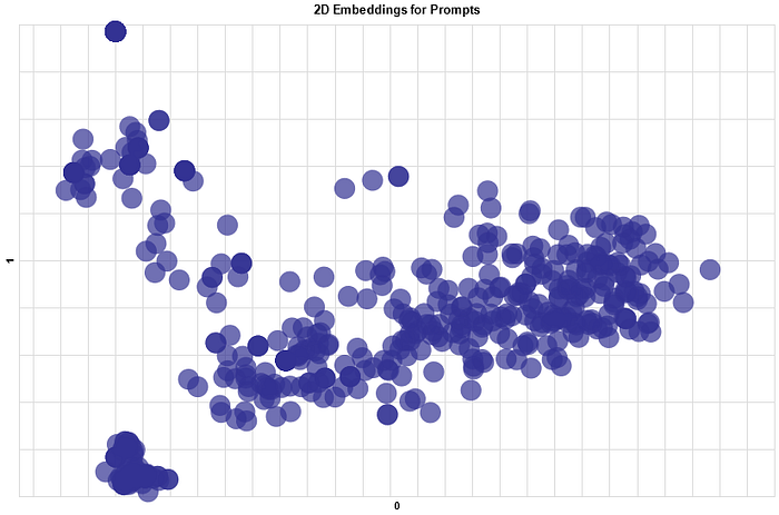
embeds = np.array(df[‘text_embeds’].tolist())
embeds_pc = get_pc(embeds,2)# Append the principal components to dataframe
df = pd.concat([df, pd.DataFrame(embeds_pc)], axis=1)# Plot the 2D embeddings on a chart
df.columns = df.columns.astype(str)
sample = 500

The scatter plot generated displays all the text prompts analyzed. Prompts that have similar meanings are closer to each other.

Semantic search for prompts

This is a technique that will allow you to find prompts that have a similar meaning to your search query. It goes beyond returning results that match keywords in the search query, by utilizing the word embeddings created above and calculating similarity based on physical distance. First, create a function that calculates a similarity score between two given word embeddings:

from sklearn.metrics.pairwise import cosine_similarity

def get_similarity(target,candidates):
  # Turn list into array
  candidates = np.array(candidates)
  target = np.expand_dims(np.array(target),axis=0)

  # Calculate cosine similarity
  sim = cosine_similarity(target,candidates)
  sim = np.squeeze(sim).tolist()
  sort_index = np.argsort(sim)[::-1]
  sort_score = [sim[i] for i in sort_index]
  similarity_scores = zip(sort_index,sort_score)

  # Return similarity scores
  return similarity_scores

Next, create word embeddings for your search query and compute the similarity scores between them and the embeddings of our prompts:

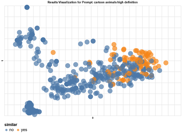
query = "cartoon animals high definition"
# embeddings of the search query
query_embeds = co.embed( model='small', texts=[query]).embeddings[0]
# similarity between the query and existing prompts
similarity = get_similarity(search_query_embeds,embeds[:sample])

print('Similar prompts:')
for idx,sim in similarity:
  if sim >= 0.30:
    df.at[idx,'similar'] = 'yes'
  else:
    df.at[idx,'similar'] = 'no'
  print(f'Similarity: {sim:.2f};',df.iloc[idx]['text'])

You can display a scatter plot to visualize the similarity of prompts. You’ll notice that similar results generally appear closer to each other.

Topic clustering

In this final section, we will explore the various topics in the prompts dataset. We will use the KMeans algorithm to create ten clusters of prompts. This algorithm is unsupervised, meaning the clusters are not labeled. However, you can plot word clouds to identify top keywords in each cluster and manually label these afterwards if you choose.

First, use scikit-learn library to set the number of clusters and fit the model:

from sklearn.cluster import KMeansn_clusters=5# Cluster the embeddings
kmeans_model = KMeans(n_clusters=n_clusters, random_state=0)
classes = kmeans_model.fit_predict(embeds).tolist()
df[‘cluster’] = (list(map(str,classes)))

Next, create word clouds for each cluster and plot them. Observe and note the main topic for each cluster:

from wordcloud import WordCloud, STOPWORDS
import matplotlib.pyplot as plt
stopwords = set(STOPWORDS)

for n in range(n_clusters):
  df_wordcloud = df.loc[df['cluster'] == str(n)]
  text = " ".join(i for i in df_wordcloud.text)
  wordcloud = WordCloud(width = 800, height = 800,
                background_color ='white',
                stopwords = stopwords,
                min_font_size = 10).generate(text)
  plt.figure(figsize = (8, 8), facecolor = None)
  plt.imshow(wordcloud)
  plt.axis("off")
  plt.tight_layout(pad = 0)
  
  # plt.show()

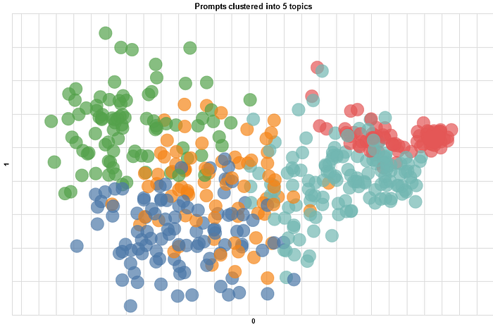
Finally, label the clusters and generate the scatter plot.

# labels the clusters after looking at keywords in each clusterdf['cluster'] = df['cluster'].replace(["0",'1','2','3','4'],
                                ['optimization','datasets', 
                                 'reasoning', 'manipulation', 
                                 'NLP'])
df.columns = df.columns.astype(str)
scatter_plot(df.iloc[:sample],'0','1',color='cluster',
             title='Prompts clustered into 5 topics')

Conclusion

Text-to-image generators present many opportunities for people in the creative fields. We have learned some of the top AI solutions currently in the market and how they work. Additionally, by analyzing a large dataset of prompts, we were able to understand how to create our own prompts and calculate the similarity of prompts. Through semantic search, we can find prompt ideas that are close to what we are looking to achieve. We can extend this analysis by adding sentiment analysis and add mood to the mix. Don’t miss the next part of this tutorial, where we are going to train a prompt generator that creates prompts for us!