Beyond Proof of Concept: Building RAG Systems That Scale
Welcome to Lesson 9 of 12 in our free course series, LLM Twin: Building Your Production-Ready AI Replica. You’ll learn how to use LLMs, vector DVs, and LLMOps best practices to design, train, and deploy a production ready “LLM twin” of yourself. This AI character will write like you, incorporating your style, personality, and voice into an LLM. For a full overview of course objectives and prerequisites, start with Lesson 1.
Lessons
- An End-to-End Framework for Production-Ready LLM Systems by Building Your LLM Twin
- Your Content is Gold: I Turned 3 Years of Blog Posts into an LLM Training
- I Replaced 1000 Lines of Polling Code with 50 Lines of CDC Magic
- SOTA Python Streaming Pipelines for Fine-tuning LLMs and RAG — in Real-Time!
- The 4 Advanced RAG Algorithms You Must Know to Implement
- Turning Raw Data Into Fine-Tuning Datasets
- 8B Parameters, 1 GPU, No Problems: The Ultimate LLM Fine-tuning Pipeline
- The Engineer’s Framework for LLM & RAG Evaluation
- Beyond Proof of Concept: Building RAG Systems That Scale
- The Ultimate Prompt Monitoring Pipeline
- [Bonus] Build a scalable RAG ingestion pipeline using 74.3% less code
- [Bonus] Build Multi-Index Advanced RAG Apps
In Lesson 9, we will focus on implementing and deploying the inference pipeline of the LLM Twin system.
First, we will design the architecture of an LLM & RAG inference pipeline based on microservices, separating the ML and RAG business logic into two layers.
Secondly, we will deploy the LLM microservice to AWS SageMaker as an inference endpoint (RESTful API).
Ultimately, we will implement the RAG business layer as a modular Python class and show you how to integrate it with a chatbot GUI using Gradio.
→ Context from previous lessons. What you must know.
As this article is part of the LLM Twin open-source course, here is what you have to know:
In Lesson 4, we populated a Qdrant vector DB with cleaned, chunked, and embedded digital data (posts, articles, and code snippets).
In Lesson 5, we implemented a retrieval module leveraging advanced RAG techniques to retrieve context.
In Lesson 7, we used Unsloth, TRL, and AWS SageMaker to fine-tune an open-source LLM publicly available on Hugging Face’s model registry.
You can use our LLM Twin at pauliusztin/LLMTwin-Meta-Llama-3.1–8B to avoid fine-tuning your model.
Don’t worry. If you don’t want to replicate the whole system, you can read this article independently from the previous lessons.
→ In this lesson, we will focus on deploying the LLM microservice to AWS SageMaker and integrating it with our RAG system.
-
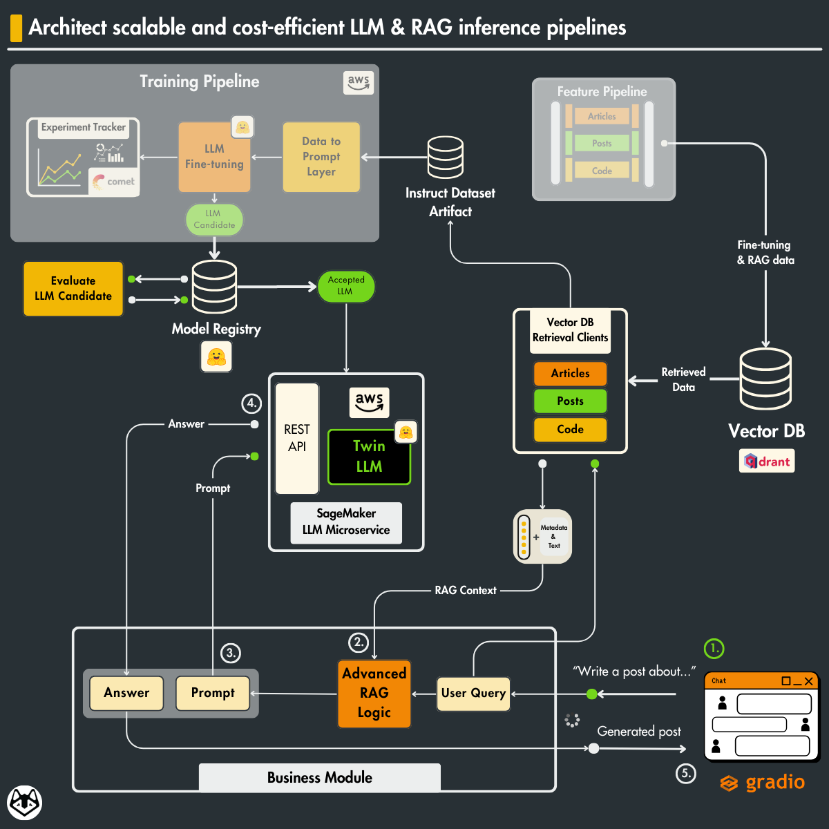
Architect scalable and cost-efficient LLM & RAG inference pipelines
Table of Contents
- Understanding the architecture of the inference pipeline
- The training vs. the inference pipeline
- Implementing the settings Pydantic class
- Deploying the fine-tuned LLM Twin to AWS SageMaker
- The RAG business module
- Deploying and running the infrence pipeline
- Implementing a chatbot UI with Gradio
🔗 Check out the code on GitHub [1] and support us with a ⭐️
1. Understanding the architecture of the inference pipeline
Our inference pipeline contains the following core elements:
- a fine-tuned LLM
- a RAG module
- a monitoring service
Let’s see how to hook these into a scalable and modular system.
The interface of the inference pipeline
As we follow the feature/training/inference (FTI) pipeline architecture, the communication between the 3 core components is clear.
Our LLM inference pipeline needs 2 things:
- a fine-tuned LLM: pulled from the model registry
- features for RAG: pulled from a vector DB (which we modeled as a logical feature store)
This perfectly aligns with the FTI architecture.
→ If you are unfamiliar with the FTI pipeline architecture, we recommend you review Lesson 1’s section on the 3-pipeline architecture.
Monolithic vs. microservice inference pipelines
Usually, the inference steps can be split into 2 big layers:
- the LLM service: where the actual inference is being done (requires special computing, such as a GPU)
- the business service: domain-specific logic (works fine on a CPU)
We can design our inference pipeline in 2 ways.
Option 1: Monolithic LLM & business service
In a monolithic scenario, we implement everything into a single service.
Pros:
- easy to implement
- easy to maintain
Cons:
- harder to scale horizontally based on the specific requirements of each component
- harder to split the work between multiple teams
- not being able to use different tech stacks for the two services
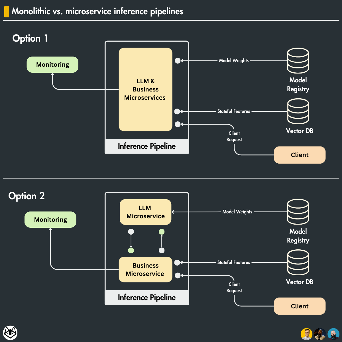
Option 2: Different LLM & business microservices
The LLM and business services are implemented as two different components that communicate with each other through the network, using protocols such as REST or gRPC.
Pros:
- each component can scale horizontally individually
- each component can use the best tech stack at hand
Cons:
- harder to deploy
- harder to maintain
Let’s focus on the “each component can scale individually” part, as this is the most significant benefit of the pattern. Usually, LLM and business services require different types of computing. For example, an LLM service depends heavily on GPUs, while the business layer can do the job only with a CPU.
As the LLM inference takes longer, you will often need more LLM service replicas to meet the demand. But remember that GPU VMs are really expensive.
By decoupling the 2 components, you will run only what is required on the GPU machine and not block the GPU VM with other computing that can quickly be done on a much cheaper machine.
Thus, by decoupling the components, you can scale horizontally as required, with minimal costs, providing a cost-effective solution to your system’s needs.
Microservice architecture of the LLM twin inference pipeline
Let’s understand how we applied the microservice pattern to our concrete LLM twin inference pipeline.
As explained in the sections above, we have the following components:
- A business microservice
- An LLM microservice
- A prompt monitoring microservice
The business microservice is implemented as a Python module that:
- contains the advanced RAG logic, which calls the vector DB and GPT-4 API for advanced RAG operations;
- calls the LLM microservice through a REST API using the prompt computed utilizing the user’s query and retrieved context
- sends the prompt and the answer generated by the LLM to the prompt monitoring microservice.
As you can see, the business microservice is light. It glues all the domain steps together and delegates the computation to other services.
The end goal of the business layer is to act as an interface for the end client. In our case, as we will ship the business layer as a Python module, the client will be a Streamlit application.
However, you can quickly wrap the Python module with FastAPI and expose it as a REST API to make it accessible from the cloud.
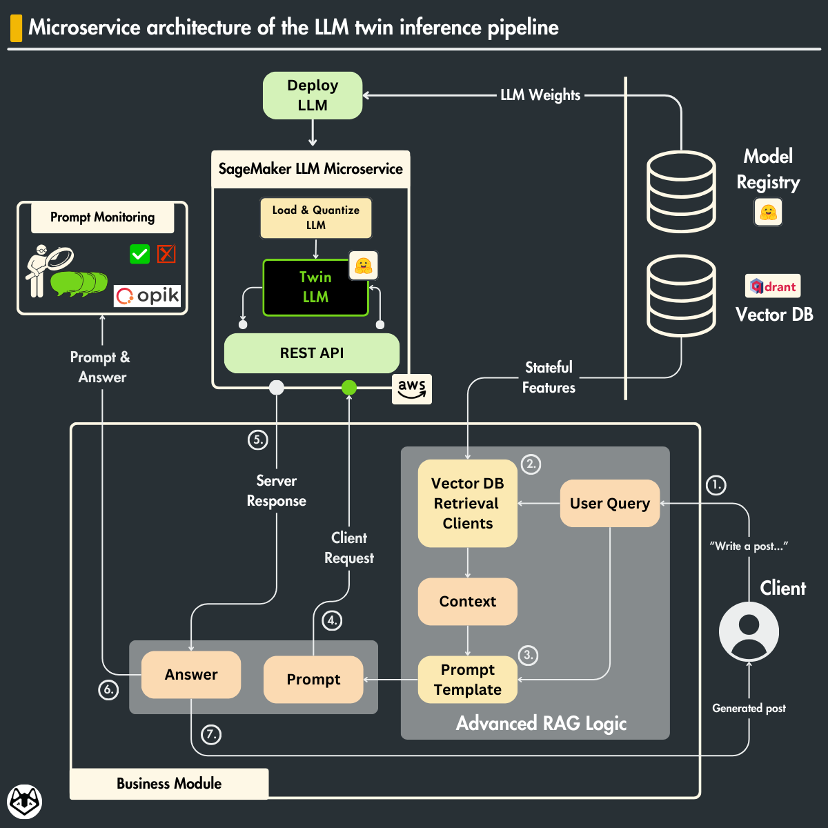
The LLM microservice is deployed on AWS SageMaker as an inference endpoint. This component is wholly niched on hosting and calling the LLM. It runs on powerful GPU-enabled machines.
How does the LLM microservice work?
- It loads the fine-tuned LLM Twin model from Hugging Face and quantizes it for lower VRAM needs.
- It exposes a REST API that takes in prompts and outputs the generated answer.
- When the REST API endpoint is called, it tokenizes the prompt, passes it to the LLM, decodes the generated tokens to a string and returns the answer.
That’s it!
The prompt monitoring microservice is based on Opik, an open-source LLM evaluation and monitoring tool powered by Comet. We will dig into the monitoring service in the next lesson.
2. The training vs. the inference pipeline
Before diving into the code, let’s quickly clarify what is the difference between the training and inference pipelines.
Along with the apparent reason that the training pipeline takes care of training while the inference pipeline takes care of inference (Duh!), there are some critical differences you have to understand.
The input of the pipeline & How the data is accessed
Do you remember our logical feature store based on the Qdrant vector DB and Comet artifacts? If not, consider checking out Lesson 6 for a refresher.
The core idea is that during training, the data is accessed from an offline data storage in batch mode, optimized for throughput and data lineage.
Our LLM twin architecture uses Comet artifacts to access, version, and track all our data.
The data is accessed in batches and fed to the training loop.
During inference, you need an online database optimized for low latency. As we directly query the Qdrant vector DB for RAG, that fits like a glove.
During inference, you don’t care about data versioning and lineage. You just want to access your features quickly for a good user experience.
The data comes directly from the user and is sent to the inference logic.
The output of the pipeline
The training pipeline’s final output is the trained weights stored in a Hugging Face model registry.
The inference pipeline’s final output is the predictions served directly to the user.
The infrastructure
The training pipeline requires more powerful machines with as many GPUs as possible.
Why? During training, you batch your data and have to hold in memory all the gradients required for the optimization steps. Because of the optimization algorithm, the training is more compute-hungry than the inference.
Thus, more computing and VRAM result in bigger batches, which means less training time and more experiments.
The inference pipeline can do the job with less computation. During inference, you often pass a single sample or smaller batches to the model.
If you run a batch pipeline, you will still pass batches to the model but don’t perform any optimization steps.
If you run a real-time pipeline, as we do in the LLM twin architecture, you pass a single sample to the model or do some dynamic batching to optimize your inference step.
Are there any overlaps?
Yes! This is where the training-serving skew comes in.
During training and inference, you must carefully apply the same preprocessing and postprocessing steps.
If the preprocessing and postprocessing functions or hyperparameters don’t match, you will end up with the training-serving skew problem.
Enough with the theory. Let’s dig into the code ↓
3. Implementing the settings Pydantic class
First, let’s understand how we defined the settings to configure the inference pipeline components.
We used pydantic_settings and inherited its BaseSettings class to define our Settings object, which takes custom values from a .env file.
This approach lets us quickly define default settings variables and load sensitive values such as the AWS and Hugging Face credentials from a .env file.
from pydantic_settings import BaseSettings, SettingsConfigDict class Settings(BaseSettings): model_config = SettingsConfigDict(env_file=".env", env_file_encoding="utf-8" ... # Settings. # LLM Model config HUGGINGFACE_ACCESS_TOKEN: str | None = None MODEL_ID: str = "pauliusztin/LLMTwin-Meta-Llama-3.1-8B" DEPLOYMENT_ENDPOINT_NAME: str = "twin" MAX_INPUT_TOKENS: int = 1536 MAX_TOTAL_TOKENS: int = 2048 MAX_BATCH_TOTAL_TOKENS: int = 2048 # AWS Authentication AWS_REGION: str = "eu-central-1" AWS_ACCESS_KEY: str | None = None AWS_SECRET_KEY: str | None = None AWS_ARN_ROLE: str | None = None ... # More settings. settings = Settings()It’s essential to notice the MODEL_ID config, which uses our fine-tuned LLM Twin by default. Change this to your Hugging Face MODEL_ID if you fine-tuned a different LLM Twin.
Also, the MAX_INPUT_TOKENS, MAX_TOTAL_TOKENS, and MAX_BATCH_TOTAL_TOKENS define the total input and output capacity of the AWS inference endpoint, such as:
- MAX_INPUT_TOKENS: Max length of input text
- MAX_TOTAL_TOKENS: Max length of the generation (including input text)
- MAX_BATCH_TOTAL_TOKENS: Limits the number of tokens that can be processed in parallel during the generation.
4. Deploying the fine-tuned LLM Twin to AWS SageMaker
The first step is to deploy our fine-tuned LLM Twin from the Hugging Face model registry as an AWS SageMaker inference endpoint.
You will see that SageMaker makes this easy.
At its core, it leverages SageMaker’s integration with Hugging Face’s model ecosystem to deploy the LLM and optimize it for inference.
More concretely, we will leverage a premade Docker image called Deep Learning Containers (DLC) [3]. We also used DLC Docker images when fine-tuning the model with SageMaker (in Lesson 7), as they are used everywhere in the Hugging Face x SageMaker combo.
These images come preinstalled with deep learning frameworks and Python libraries such as Transformers, Datasets, and Tokenizers.
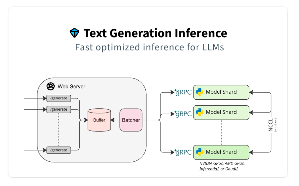
But we are primarily interested in the Hugging Face Inference DLC, which comes with a pre-written serving stack that drastically lowers the technical bar of deep learning serving, which is based on the Text Generation Inference (TGI) server [2] (also made by Hugging Face).
TGI offers goodies such as:
- Tensor parallelism for faster inference on multiple GPUs;
- Token streaming;
- Continuous batching of incoming requests for increased total throughput;
- Optimizations through using Flash Attention and Paged Attention;
- Quantization with bitsandbytes and GPT-Q;
…and more!
from config import settings from sagemaker.huggingface import HuggingFaceModel, get_huggingface_llm_image_uri def main() -> None: assert settings.HUGGINGFACE_ACCESS_TOKEN, "HUGGINGFACE_ACCESS_TOKEN is required." env_vars = { "HF_MODEL_ID": settings.MODEL_ID, "SM_NUM_GPUS": "1", # Number of GPU used per replica. "HUGGING_FACE_HUB_TOKEN": settings.HUGGINGFACE_ACCESS_TOKEN, "MAX_INPUT_TOKENS": str(settings.MAX_INPUT_TOKENS), "MAX_TOTAL_TOKENS": str(settings.MAX_TOTAL_TOKENS), "MAX_BATCH_TOTAL_TOKENS": str(settings.MAX_BATCH_TOTAL_TOKENS), "MESSAGES_API_ENABLED": "true", "HF_MODEL_QUANTIZE": "bitsandbytes", } These settings control everything from the model’s identity and GPU allocation to token limits and API behavior.
By setting the MESSAGES_API_ENABLED variable to true, we enabled a protocol similar to the one used with the OpenAI REST API client.
The quantization is set to use bitsandbytes, compressing the LLM to 8bits for lower VRAM requirements and inference time (latency).
image_uri = get_huggingface_llm_image_uri("huggingface", version="2.2.0") model = HuggingFaceModel( env=env_vars, role=settings.AWS_ARN_ROLE, image_uri=image_uri ) model.deploy( initial_instance_count=1, instance_type="ml.g5.2xlarge", container_startup_health_check_timeout=900, endpoint_name=settings.DEPLOYMENT_ENDPOINT_NAME, ) The final stage involves the actual model deployment configuration and execution. The DLC Docker image is retrieved as an ECR URL through the get_huggingface_llm_image_uri() function.
Afterward, the code initializes a SageMaker HuggingFaceModel instance with the specified environment variables and AWS role, then deploys it to a g5.2xlarge instance.
The deployment includes a generous health check timeout of 15 minutes to ensure proper model loading and initialization.
As we use an 8B LLM with quantization using a g5.2xlarge instance with an A10G Nvidia GPU that has 24GB VRAM is enough to deploy our model.
SageMaker supports autoscaling to handle traffic spikes and idle time to optimize costs while offering the best experience to the clients (not implemented in this lesson, though).
Now, we can access the deployed model as easily as:
from sagemaker.huggingface.model import HuggingFacePredictor sagemaker_inference_endpoint = HuggingFacePredictor( endpoint_name=settings.DEPLOYMENT_ENDPOINT_NAME, sagemaker_session=sagemaker.Session(), ) answer = sagemaker_inference_endpoint.predict(...) But more on this in the next section.
→ Full code in the inference_pipeline/aws/deploy_sagemaker_endpoint.py file.
5. The RAG business module
We will define the RAG business module under the LLMTwin class.
All the LLM Twin logic represents our business layer.
We don’t have to introduce the word “business” in the class naming convention. What we presented so far was used to separate the concerns between the LLM microservice and business layers.
The LLMTwin class, at its core, manages the connection to the Sagemaker endpoint and RAG business logic, with support for both real and mock interactions for testing purposes.
class LLMTwin: def __init__(self, mock: bool = False) -> None: self._mock = mock self._llm_endpoint = self.build_sagemaker_predictor() self.prompt_template_builder = InferenceTemplate() def build_sagemaker_predictor(self) -> HuggingFacePredictor: return HuggingFacePredictor( endpoint_name=settings.DEPLOYMENT_ENDPOINT_NAME, sagemaker_session=sagemaker.Session(), ) The generation() method orchestrates the entire inference process. It begins by creating appropriate templates based on whether RAG is enabled.
When RAG is active, it leverages our VectorRetriever module (implemented in Lesson 5) to fetch and rerank relevant context, which is then incorporated into the prompt template variables.
def generate( self, query: str, enable_rag: bool = False, sample_for_evaluation: bool = False, ) -> dict: system_prompt, prompt_template = self.prompt_template_builder.create_template( enable_rag=enable_rag ) prompt_template_variables = {"question": query} if enable_rag is True: retriever = VectorRetriever(query=query) hits = retriever.retrieve_top_k( k=settings.TOP_K, to_expand_to_n_queries=settings.EXPAND_N_QUERY ) context = retriever.rerank(hits=hits, keep_top_k=settings.KEEP_TOP_K) prompt_template_variables["context"] = context else: context = None messages, input_num_tokens = self.format_prompt( system_prompt, prompt_template, prompt_template_variables ) answer = self.call_llm_service(messages=messages) The prompt formatting logic ensures that inputs stay within token limits by truncating content while preserving the system prompt. This careful management of token counts is essential for reliable operation with token-constrained language models.
Note how we formatted the messages in the same format as when using the OpenAI client. We can easily add memory using the messages API format, such as handling the chat history.
def format_prompt( self, system_prompt, prompt_template: PromptTemplate, prompt_template_variables: dict, ) -> tuple[list[dict[str, str]], int]: prompt = prompt_template.format(**prompt_template_variables) num_system_prompt_tokens = compute_num_tokens(system_prompt) prompt, prompt_num_tokens = truncate_text_to_max_tokens( prompt, max_tokens=settings.MAX_INPUT_TOKENS - num_system_prompt_tokens ) total_input_tokens = num_system_prompt_tokens + prompt_num_tokens messages = [ {"role": "system", "content": system_prompt}, {"role": "user", "content": prompt}, ] Finally, the actual interaction with the language model is handled through a Sagemaker endpoint.
The system supports a mock mode for testing. Still, in production, it makes a real call with carefully tuned parameters for temperature and top-p sampling, ensuring consistent and high-quality responses.
def call_llm_service(self, messages: list[dict[str, str]]) -> str: if self._mock is True: return "Mocked answer." answer = self._llm_endpoint.predict( data={ "messages": messages, "parameters": { "max_new_tokens": settings.MAX_TOTAL_TOKENS - settings.MAX_INPUT_TOKENS, "temperature": 0.01, "top_p": 0.6, "stop": ["<|eot_id|>"], "return_full_text": False, }, } ) answer = answer["choices"][0]["message"]["content"].strip() When not using RAG, our inference prompt template follows the Alpaca format:
class InferenceTemplate(BasePromptTemplate): simple_system_prompt: str = """ You are an AI language model assistant. Your task is to generate a cohesive and concise response based on the user's instruction by using a similar writing style and voice. """ simple_prompt_template: str = """ ### Instruction: {question} """ …and when using RAG, it follows the same format but enforces the LLM to respond based on the provided context:
class InferenceTemplate(BasePromptTemplate): ... rag_system_prompt: str = """ You are a specialist in technical content writing. Your task is to create technical content based on the user's instruction given a specific context with additional information consisting of the user's previous writings and his knowledge. Here is a list of steps that you need to follow in order to solve this task: Step 1: You need to analyze the user's instruction. Step 2: You need to analyze the provided context and how the information in it relates to the user instruction. Step 3: Generate the content keeping in mind that it needs to be as cohesive and concise as possible based on the query. You will use the users writing style and voice inferred from the user instruction and context. First try to answer based on the context. If the context is irrelevant answer with "I cannot answer your question, as I don't have enough context." """ rag_prompt_template: str = """ ### Instruction: {question} ### Context: {context} """ def create_template(self, enable_rag: bool = True) -> tuple[str, PromptTemplate]: if enable_rag is True: return self.rag_system_prompt, PromptTemplate( template=self.rag_prompt_template, input_variables=["question", "context"], ) return self.simple_system_prompt, PromptTemplate( template=self.simple_prompt_template, input_variables=["question"] ) Now, the LLMTwin module can easily be instantiated as required:
- In a FastAPI webserver.
- In a Gradio/Streamlit dashboard (which we will do in this lesson).
- In an evaluation pipeline.
- In a batch or async pipeline.
For example, we can use it as easy as:
inference_endpoint = LLMTwin(mock=False) query = """ Hello I am Paul Iusztin. Could you draft an article paragraph discussing RAG? I'm particularly interested in how to design a RAG system. """ response = inference_endpoint.generate( query=query, enable_rag=True, sample_for_evaluation=False ) Further, we can improve it by adding streaming or async support to optimize the inference process.
→ Full code in the inference_pipeline/llm_twin.py file.
6. Deploying and running the inference pipeline
The last step is understanding how to run all the code from above.
The first step is to ensure that your AWS setup is ready. You need to fill in the following environment variables in your .env file:
AWS_ARN_ROLE=str AWS_REGION=eu-central-1 AWS_ACCESS_KEY=str AWS_SECRET_KEY=str It’s pretty easy. It’s just a 2 step process. All the details on how to do it are in our repo’s INSTALL_AND_USAGE document.
Also, if enabling RAG, you must ensure that your Qdrant vector DB is running and populated with relevant data. To spin it up locally, run:
make local-start
You can find a quick guide on how to set everything up in our INSTALL_AND_USAGE document.
Next, you can deploy the LLM microservice to SageMaker by running:
make deploy-inference-pipeline
Now, you can test the inference pipeline by running:
make call-inference-pipeline
Ultimately, you can stop the AWS SageMaker inference endpoint and clean up all the resources by running the following:
make delete-inference-pipeline-deployment
Find step-by-step instructions on installing and running the entire course in our INSTALL_AND_USAGE document from the repository.
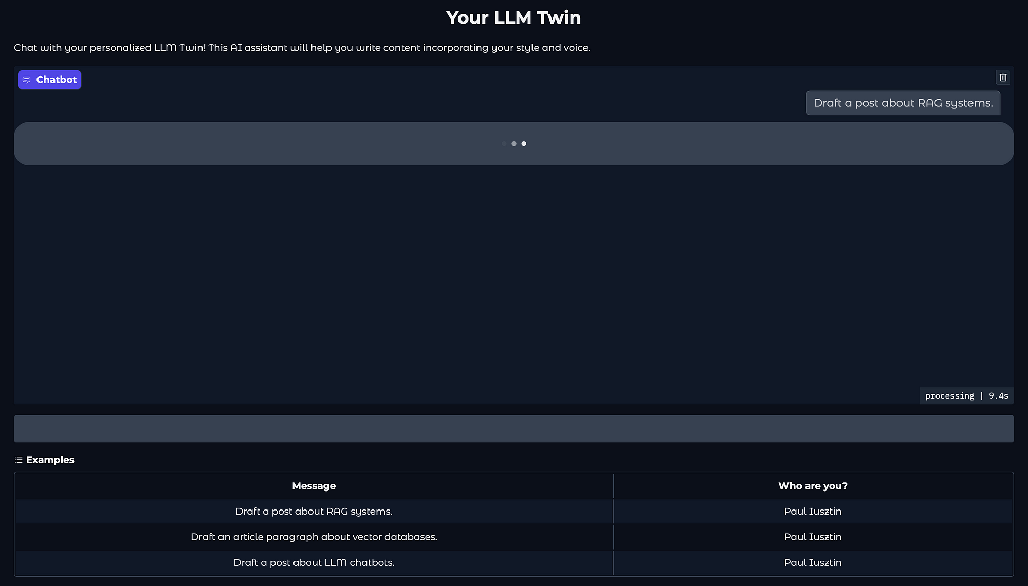
7. Implementing a chatbot UI with Gradio
Now, let’s see how we can test our inference pipeline in a Gradio chat GUI.
The code is straightforward as Gradio provides the ChatInterface abstraction, as seen in the code snippet below:
import gradio as gr demo = gr.ChatInterface( predict, textbox=gr.Textbox( placeholder="Chat with your LLM Twin", label="Message", container=False, scale=7, ), additional_inputs=[ gr.Textbox( "Paul Iusztin", label="Who are you?", ) ], title="Your LLM Twin", description=""" Chat with your personalized LLM Twin! This AI assistant will help you write content incorporating your style and voice. """, theme="soft", examples=[ [ "Draft a post about RAG systems.", "Paul Iusztin", ], ... ], cache_examples=False, ) if __name__ == "__main__": demo.queue().launch(server_name="0.0.0.0", server_port=7860, share=True) As we’ve built a modular inference pipeline under the LLMTwin class, we can hook all our AI logic to the Gradio UI with a few lines of code:
 from inference_pipeline.llm_twin import LLMTwin

llm_twin = LLMTwin(mock=False)


def predict(message: str, history: list[list[str]], author: str) -> str:
    """
    Generates a response using the LLM Twin, simulating a conversation with your digital twin.

    Args:
        message (str): The user's input message or question.
        history (List[List[str]]): Previous conversation history between user and twin.
        about_me (str): Personal context about the user to help personalize responses.

    Returns:
        str: The LLM Twin's generated response.
    """

    query = f"I am {author}. Write about: {message}"
    response = llm_twin.generate(
        query=query, enable_rag=True, sample_for_evaluation=False
    )

    return response["answer"]
Now, we can run the following:
make local-start-ui
…and BOOM! we have a nice, clean UI to play around with our LLM Twin model.
Full code at inference_pipeline/ui.py.
Conclusion
In this lesson of the LLM Twin course, you learned to build a scalable inference pipeline for serving LLMs and RAG systems.
First, you learned how to architect an inference pipeline by understanding the difference between monolithic and microservice architectures. We also highlighted the difference in designing the training and inference pipelines.
Secondly, we showed you how to deploy and run the LLM Twin microservice on AWS SagaMaker as an inference endpoint.
Ultimately, we walked you through implementing the RAG business module and LLMTwin class. We showed how easily you can port it to various services, such as a Gradio chat GUI.
Continue the course with Lesson 10 on monitoring the prompt traces (generated by the inference pipeline) and build a monitoring evaluation pipeline using Opik.
🔗 Consider checking out the GitHub repository [1] and support us with a ⭐️
References
References
Literature
[1] Your LLM Twin Course — GitHub Repository (2024), Decoding ML GitHub Organization
Images
If not otherwise stated, all images are created by the author.
Related Articles