Machine learning is a subset of artificial intelligence that employs statistical algorithms and other methods to visualize, analyze and forecast data. Generally, machine learning is broken down into two subsequent categories based on certain properties of the data used: supervised and unsupervised.

Supervised learning algorithms refer to those that require training datasets with labels attached to the features. Unsupervised learning algorithms, on the other hand, make use of mathematical formulas that find patterns in unlabelled data, often by identifying clusters of data with similar (but independent) features. In this article, we will discuss different clustering algorithms and how to evaluate their results. Let’s get started!

What is Clustering?

Clustering (sometimes referred to as cluster analysis) is an unsupervised machine learning technique used to identify and group similar data points within a larger, unlabelled dataset. It refers to the process of finding a structure or pattern inside an otherwise unstructured dataset.

The four main types of clustering include:

• Centroid-based Clustering (e.g., K-Means Clustering)
• Density-based Clustering (e.g., DBSCAN)
• Distribution-based Clustering (e.g., Gaussian Mixture Models, or GMMs)
• Hierarchical Clustering (e.g., Agglomerative, Divisive)

In this article we will explore K-means clustering, hierarchical clustering, and DBSCAN, as these are some of the most common (and effective) methods used currently, but it’s good to be aware that there are other methods out there as well.

1. K-Means Clustering

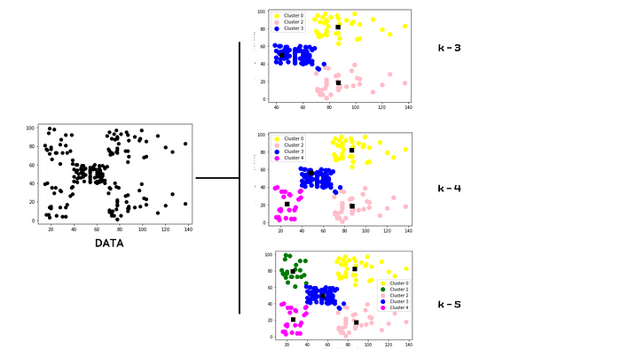
K-means clustering is an unsupervised machine learning algorithm that groups unlabeled data into k number clusters, where k is a user-defined integer. K-means is an iterative algorithm that makes use of cluster centroids to divide the data in a way that groups similar data into groups.

K-means clustering starts by taking k random points, and marks these points as centroids of k clusters. It then calculates the Euclidean distance for each remaining data point from each of those centroids and assigns each data point to its closest cluster (based on the Euclidean distance from the centroid). Once a new point is added to the cluster, it recalculates the centroid by taking the mean of all the vectors inside the group, and then recursively calculates distance again. Then, the new centroid is recalculated, and this is repeated until all data points are assigned to a cluster.

In order for K-means clustering to be effective, however, it is imperative to first determine the optimal value for k. There are various techniques for doing so, but one of the most effective is through simple data visualization. We will also cover a couple of other methods, however, in examples later on.

2. Hierarchical Clustering

Hierarchical clustering is another type of unsupervised clustering algorithm, in which we create a hierarchy of clusters in the form of a tree, also referred to as a dendrogram. Hierarchical clustering also automatically finds patterns by dividing data into n clusters. However, in this case, there is no need to define the number of clusters (the algorithm will determine this for you).

There are two main approaches to hierarchical clustering: agglomerative and divisive. In agglomerative clustering, we consider each data point as a single cluster, and then combine these clusters until we are left with one group (the full dataset). Divisive hierarchical clustering, on the other hand, begins with the whole dataset (considered as one single cluster), which is then partitioned into less similar clusters until each individual data point becomes its own unique cluster.

3. DBSCAN Clustering

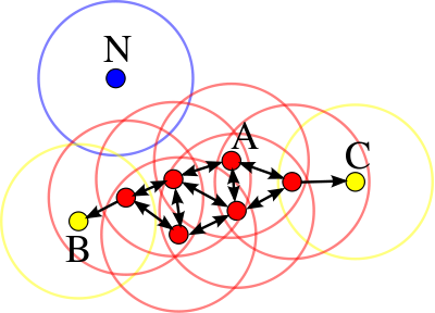
DBSCAN stands for density-based spatial clustering of application with noise. DBSCAN clustering works upon a simple assumption that a data point belongs to a cluster if it is closer to many data points of that cluster, rather than any single point. It requires two parameters for dividing data into groups: epsilon and min_points. epsilon specifies how close one point should be to another in order to consider it part of the cluster, while min_points determines the minimum number of data points required to form a cluster.

One of the biggest advantages of DBSCAN clustering is that it is very robust to outliers and doesn’t require information about the cluster size for training.

Struggling to track and reproduce complex experiment parameters? Artifacts are just one of the many tools in the Comet toolbox to help ease model management. Read our PetCam scenario to learn more.

Building a Clustering Model

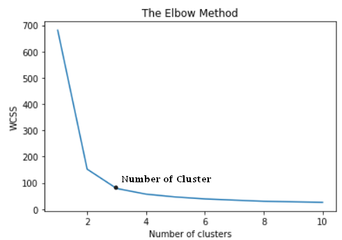
We are going to make use of the K-means clustering algorithm to cluster different iris flower species into clusters, using the famous iris dataset. To determine the correct number of clusters we will make use of the elbow method. The dataset we are using is located in the sklearn dataset class.

from sklearn import datasets
df = datasets.load_iris()
X = df['data']
y = df['target']               # not needed for clustering

X will contain information about sepal width, sepal length, and petal width whereas y will contain information regarding the type of flower species. We will only use X, and try to divide the dataset into different flower species clusters using K-means instead. Below, we use the elbow method to find the value of k.

from sklearn.cluster import KMeanswcss = []
for i in range(1, 11):
    kmeans = KMeans(n_clusters = i, init = 'k-means++', 
                random_state = 42)
    kmeans.fit(X)
    wcss.append(kmeans.inertia_)
plt.plot(range(1, 11), wcss)
plt.title('The Elbow Method')
plt.xlabel('Number of clusters')
plt.ylabel('WCSS')
plt.show()

The elbow method has given us an optimal value of k that is 3. Let’s use this value to build a model.

from sklearn.cluster import KMeans
Kmean = KMeans(n_clusters=3)
Kmean.fit(X)## Predictions
y_pred = Kmean.predict(X)

Now that we have our labels and predictions let’s evaluate this model to find out well it performed!

Evaluation Metrics For Clustering-Based Models

1. Silhouette Score

• The silhouette score is a metric used to calculate the goodness of fit of a clustering algorithm, but can also be used as a method for determining an optimal value of k (see here for more).
• It is calculated by taking the mean distance from intra-cluster and nearest cluster samples.
• Its value ranges from -1 to 1.
• A value of 0 indicates clusters are overlapping and either the data or the value of k is incorrect.
• 1 is the ideal value and indicates that clusters are very dense and nicely separated.
• A negative value indicates elements have likely been assigned to the wrong clusters.
• The closer the value of the silhouette score to 1 the better-separated the clusters.

from sklearn.metrics import silhouette_score
silhouette_score(X,y_pred)
--------------------------------
0.55"""
silhouette score is 0.55 which is acceptable and shows clusters are not overlapping.
"""

2. Calinski Harabaz Index

• It is also known as the Variance Ratio Criterion.
• Calinski Harabaz Index is defined as the ratio of the sum of between-cluster dispersion and of within-cluster dispersion.
• The higher the index the more separable the clusters.

from sklearn.metrics import calinski_harabasz_score
calinski_harabasz_score(X,y_pred)
---------------------------------------------
561.62775

3. Davies Bouldin index

• The Davies–Bouldin index (DBI), introduced by David L. Davies and Donald W. Bouldin in 1979, is another metric for evaluating clustering algorithms.
• The Davies Bouldin index is defined as the average similarity measure of each cluster with its most similar cluster, where similarity is the ratio of within-cluster distances to between-cluster distances.
• The minimum value of the DB Index is 0, whereas a smaller value (closer to 0) represents a better model that produces better clusters.

from sklearn.metrics import davies_bouldin_score
davies_bouldin_score(X,y_pred)
-------------------------------------------
0.6619

Based on the above evaluation scores we can conclude that our model is a decent performer.

Conclusion

It is always a better idea to evaluate your machine learning models before making decisions based on them. Metric evaluation is an easy-to-interpret solution for checking the performance of the model.