Estimating Uncertainty in Machine Learning Models – Part 2

 

You can check out part 1 of this series here

In part 1 of this series, we discussed the sources of uncertainty in machine learning models, and techniques to quantify uncertainty in the parameters, and predictions of a simple linear regression model.

The techniques described in the last post, such as bootstrapping, have their limits in cases where fitting a model takes a significant amount time, due to the size of the dataset, or the size of the model, such as in Neural Networks.

In this part of our series we’re going to look at a technique that can provide uncertainty estimates at prediction time for any Neural Network architecture, without making any changes to how the network is trained.

Prediction Intervals using Dropout

Dropout is commonly thought of as an empirical technique to prevent overfitting in deep learning models. Dropout involves ignoring a random subset of neurons in a network layer at every batch evaluation. We can think of this as approximating the training of an ensemble of networks, since every weight update is changing a subset of parameters in the network. We can leverage this approximating behavior at prediction time.

Normally, Dropout is only used during the training phase of the network. However, by leaving it on during prediction, we end up with the equivalent of an ensemble of subnetworks, within our single larger network, that have slightly different views of the data. If we create a set of T predictions from our model, we can use the mean, and variance of this prediction set to estimate our uncertainty.

Let’s use the the Auto MPG dataset provided in the Tensorflow Keras documentation to demonstrate this approach. We’re going to use the dataset after applying all the preprocessing steps mentioned in the linked documentation.

The amazing thing about this approach is that it requires a very minimal change to your code to

Turning Dropout on during prediction is easy. Simply set the training argument in the call of the Dropout layer to True.

from keras.models import Model
from keras.layers import Input, Dense, Dropout

dropout_rate = 0.25

def model_fn():
    inputs = Input(shape=(9,))
    x = Dense(64, activation='relu')(inputs)
    x = Dropout(dropout_rate)(x, training=True)
    x = Dense(64, activation='relu')(x)
    x = Dropout(dropout_rate)(x, training=True)
    outputs = Dense(1)(x)
    
    model = Model(inputs, outputs)
    model.compile(loss="mean_squared_error", optimizer='adam')
    
    return model

We can now use it to make predictions in the following way

import numpy as np

predictions = []

sample_size = 100
for t in range(sample_size):
    predictions.append(model.predict(normed_test_data))

prediction_df = pd.DataFrame()

pred_array = np.array(predictions)
prediction_df['mean'] = pred_array.mean(axis=0).reshape(-1,)
prediction_df['std'] = pred_array.std(axis=0).reshape(-1,)

Let’s plot our predictions, along with our intervals, against our actual target values to see how we did.

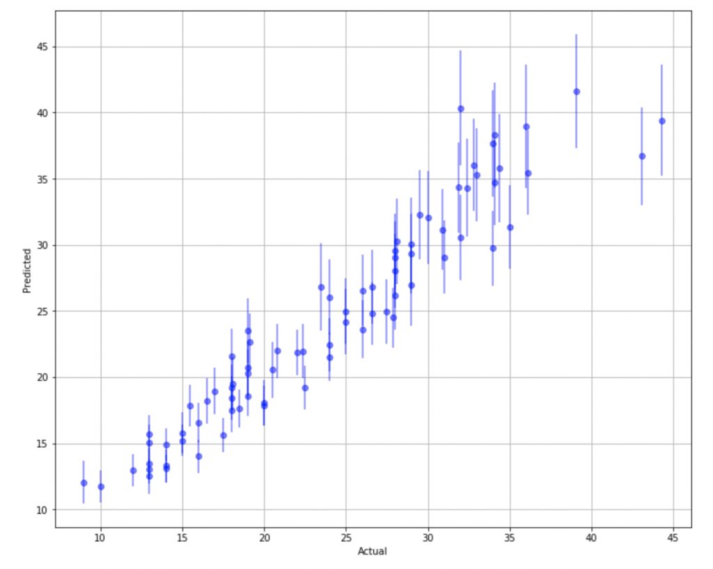
Notice how predictions that do not match well with the actual values have very wide prediction intervals. This shows us that our model is not able to adequately capture information about the features that produce these responses.

Of course our interval estimates are sensitive to the size of T, and the value p that controls the proportion of neurons that are dropped in a particular layer. To assess the affects of these parameters on our intervals, we should first select a metric that helps us capture the quality of our intervals. Prediction Interval Coverage Probability (PICP) and Mean Prediction Interval Width are two such metrics. PICP tells us the percentage of time an interval contains the actual value of the prediction, while MPIW gives us the average width of a predicted interval.

Our goal is to maximize PICP, while minimizing MPIW in order to get high quality intervals. Let’s run a few trials with different values of p to see how it affects our metrics

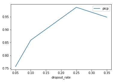
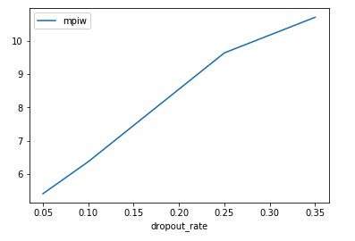
So in our case, increasing our dropout rate causes an increase in both PICP and MPIW. This does intuitively make sense. The large the number of neurons being dropped out of the network, the higher the variance in the output. This would lead to larger average intervals that would capture our target value.

Now lets take a look at the effect of our sample size, T . We’re going to keep a fix our dropout rate at 0.10 in both layers and vary our sample size.

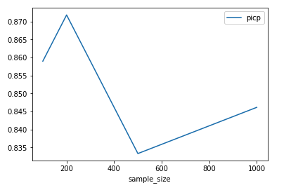
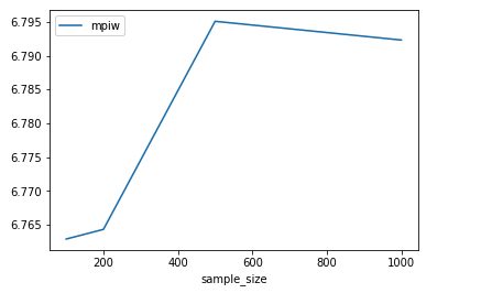
In our particular case, it seems that our interval metrics are fairly independent of the sample size. We do not see dramatic changes in either one of them as we increase the sample size from 100 to 1000.

Conclusion

We’ve looked at how we can use Dropout as a way to estimate of model uncertainty at prediction time. This technique is formally known as MC Dropout, and was developed by Yarin Gal, while he was completing his PhD at Cambridge.

This approach circumvents the computational bottlenecks associated with having to train an ensemble of Neural Networks in order to estimate predictive uncertainty.

One shortcoming of this approach, is that it requires making T number of predictions for every new datapoint. Depending on the use case this might not be feasible for real time inference (e.g in self driving cars). The other limitation is that you must use Dropout as your regularizer, which may not always apply to your use case.

In part 3 of our series on uncertainty, we’ll look at approaches that can give us an estimate of uncertainty from a single prediction, and compare it to the methods seen so far.

---

Want to stay in the loop? Subscribe to the Comet Newsletter for weekly insights and perspective on the latest ML news, projects, and more.