In the last post, you created a 2-layer neural network from scratch and now have a better understanding of how neural networks work.

In this second part, you’ll use your network to make predictions, and also compare its performance to two standard libraries (scikit-learn and Keras).

Specifically, you’ll learn how to:

• Train and test the neural network
• Build a 2-layer neural network using scikit-learn
• Build a 2-layer neural network using Keras

👉🏽 Full code in Google Colab here.

Training and Testing the Neural Network

In case you’ve forgotten what your network looks like, here’s the code:

class NeuralNet():
    '''
    A two layer neural network
    '''
        
    def __init__(self, layers=[13,8,1], learning_rate=0.001, iterations=100):
        self.params = {}
        self.learning_rate = learning_rate
        self.iterations = iterations
        self.loss = []
        self.sample_size = None
        self.layers = layers
        self.X = None
        self.y = None
                
    def init_weights(self):
        '''
        Initialize the weights from a random normal distribution
        '''
        np.random.seed(1) # Seed the random number generator
        self.params["W1"] = np.random.randn(self.layers[0], self.layers[1]) 
        self.params['b1']  =np.random.randn(self.layers[1],)
        self.params['W2'] = np.random.randn(self.layers[1],self.layers[2]) 
        self.params['b2'] = np.random.randn(self.layers[2],)
    
    def relu(self,Z):
        '''
        The ReLu activation function is to performs a threshold
        operation to each input element where values less 
        than zero are set to zero.
        '''
        return np.maximum(0,Z)

    def dRelu(self, x):
        x[x<=0] = 0
        x[x>0] = 1
        return x

    def eta(self, x):
      ETA = 0.0000000001
      return np.maximum(x, ETA)


    def sigmoid(self,Z):
        '''
        The sigmoid function takes in real numbers in any range and 
        squashes it to a real-valued output between 0 and 1.
        '''
        return 1/(1+np.exp(-Z))

    def entropy_loss(self,y, yhat):
        nsample = len(y)
        yhat_inv = 1.0 - yhat
        y_inv = 1.0 - y
        yhat = self.eta(yhat) ## clips value to avoid NaNs in log
        yhat_inv = self.eta(yhat_inv) 
        loss = -1/nsample * (np.sum(np.multiply(np.log(yhat), y) + np.multiply((y_inv), np.log(yhat_inv))))
        return loss

    def forward_propagation(self):
        '''
        Performs the forward propagation
        '''
        
        Z1 = self.X.dot(self.params['W1']) + self.params['b1']
        A1 = self.relu(Z1)
        Z2 = A1.dot(self.params['W2']) + self.params['b2']
        yhat = self.sigmoid(Z2)
        loss = self.entropy_loss(self.y,yhat)

        # save calculated parameters     
        self.params['Z1'] = Z1
        self.params['Z2'] = Z2
        self.params['A1'] = A1

        return yhat,loss

    def back_propagation(self,yhat):
        '''
        Computes the derivatives and update weights and bias according.
        '''
        y_inv = 1 - self.y
        yhat_inv = 1 - yhat

        dl_wrt_yhat = np.divide(y_inv, self.eta(yhat_inv)) - np.divide(self.y, self.eta(yhat))
        dl_wrt_sig = yhat * (yhat_inv)
        dl_wrt_z2 = dl_wrt_yhat * dl_wrt_sig

        dl_wrt_A1 = dl_wrt_z2.dot(self.params['W2'].T)
        dl_wrt_w2 = self.params['A1'].T.dot(dl_wrt_z2)
        dl_wrt_b2 = np.sum(dl_wrt_z2, axis=0, keepdims=True)

        dl_wrt_z1 = dl_wrt_A1 * self.dRelu(self.params['Z1'])
        dl_wrt_w1 = self.X.T.dot(dl_wrt_z1)
        dl_wrt_b1 = np.sum(dl_wrt_z1, axis=0, keepdims=True)

        #update the weights and bias
        self.params['W1'] = self.params['W1'] - self.learning_rate * dl_wrt_w1
        self.params['W2'] = self.params['W2'] - self.learning_rate * dl_wrt_w2
        self.params['b1'] = self.params['b1'] - self.learning_rate * dl_wrt_b1
        self.params['b2'] = self.params['b2'] - self.learning_rate * dl_wrt_b2

    def fit(self, X, y):
        '''
        Trains the neural network using the specified data and labels
        '''
        self.X = X
        self.y = y
        self.init_weights() #initialize weights and bias


        for i in range(self.iterations):
            yhat, loss = self.forward_propagation()
            self.back_propagation(yhat)
            self.loss.append(loss)

    def predict(self, X):
        '''
        Predicts on a test data
        '''
        Z1 = X.dot(self.params['W1']) + self.params['b1']
        A1 = self.relu(Z1)
        Z2 = A1.dot(self.params['W2']) + self.params['b2']
        pred = self.sigmoid(Z2)
        return np.round(pred) 

    def acc(self, y, yhat):
        '''
        Calculates the accutacy between the predicted valuea and the truth labels
        '''
        acc = int(sum(y == yhat) / len(y) * 100)
        return acc


    def plot_loss(self):
        '''
        Plots the loss curve
        '''
        plt.plot(self.loss)
        plt.xlabel("Iteration")
        plt.ylabel("logloss")
        plt.title("Loss curve for training")
        plt.show()

To train and test the network, you’ll read in the heart disease dataset, preprocess it like you would in any other machine learning task, specifically, you’ll:

• Split the data into train and test sets,
• Standardize it using StandardScaler,
• Initialize a model from your NeuralNetwork class, and finally,
• Train and predict with the Model

import numpy as np
import warnings
warnings.filterwarnings("ignore") #suppress warnings
import matplotlib.pyplot as plt
from sklearn.model_selection import train_test_split
from sklearn.preprocessing import StandardScaler

#convert imput to numpy arrays
X = heart_df.drop(columns=['heart_disease'])

#replace target class with 0 and 1 
#1 means "have heart disease" and 0 means "do not have heart disease"
heart_df['heart_disease'] = heart_df['heart_disease'].replace(1, 0)
heart_df['heart_disease'] = heart_df['heart_disease'].replace(2, 1)

y_label = heart_df['heart_disease'].values.reshape(X.shape[0], 1)

#split data into train and test set
Xtrain, Xtest, ytrain, ytest = train_test_split(X, y_label, test_size=0.2, random_state=2)

#standardize the dataset
sc = StandardScaler()
sc.fit(Xtrain)
Xtrain = sc.transform(Xtrain)
Xtest = sc.transform(Xtest)

print(f"Shape of train set is {Xtrain.shape}")
print(f"Shape of test set is {Xtest.shape}")
print(f"Shape of train label is {ytrain.shape}")
print(f"Shape of test labels is {ytest.shape}")

In the code block above, first, you get the training data, excluding the label—this is done with the drop function. The drop function removes the specified column from the dataset and returns the remaining features. Next, you saved the label to a variable calledy_label.

Next, you split the data into train and test set, with the test set taking 10 percent of the overall data. Then, you standardize the dataset. Standardization is important when working with neural networks, as it has a serious effect on the training time and network performance.

In the next code section, you’ll initialize the neural network and train it using the fit function.

nn = NeuralNet() # create the NN model
nn.fit(Xtrain, ytrain) #train the model

Here, you initialize the neural network with the default parameters:

• layers ==> [13,8,1]
• learning_rate ==> 0.001
• iterations ==> 100

Then, you passed in the training data (Xtrain,ytrain) to the fit method. This is the training phase of the model.

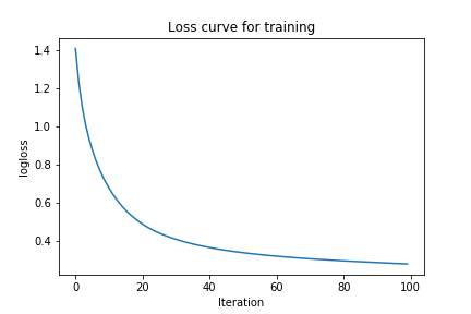
Now that you’re done training, let’s plot the loss using the handy plot_lossfunction in the NeuralNetwork class:

nn.plot_loss()

You can see that the loss starts pretty high, then quickly goes down, and starts approaching zero. This gives you an insight into how the network learns. Now, let’s try increasing the learning rate and the size of the hidden layer, and see how it affects the loss.

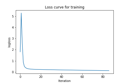
nn = NeuralNet(layers=[13,10,1], learning_rate=0.01, iterations=500) # create the NN model
nn.fit(Xtrain, ytrain) #train the model
nn.plot_loss()

You can clearly see that the loss is lower than the previous one. So these sets of parameters might actually be doing better than the first. To confirm this, let’s show the accuracy on both the train and test set.

For the first Architecture, we have the following accuracies:

train_pred = nn.predict(Xtrain)
test_pred = nn.predict(Xtest)

print("Train accuracy is {}".format(nn.acc(ytrain, train_pred)))
print("Test accuracy is {}".format(nn.acc(ytest, test_pred)))

For the second network, I had the same set of accuracies. This suggests that the second model is overfitting the data and the first model is actually better.

And just so you know, those are pretty great accuracies for a Neural Network you built from scratch!

Working with Python Libraries

Just to spice it up, let’s compare your implementation with standard libraries like Keras and scikit-learn. If you don’t have these libraries installed on your machine, you either have to install them or use Google Colab for this section.

A 2-Layer Neural Network with scikit-learn

The MLPClassifier in the scikit-learn package contains an implementation of a neural network. To use it, first, you have to import it from the sklearn.neural_network class, and initialize the architecture:

from sklearn.neural_network import MLPClassifier
from sklearn.metrics import accuracy_score

sknet = MLPClassifier(hidden_layer_sizes=(8), learning_rate_init=0.001, max_iter=100)

Notice that you specify just the number of hidden nodes when using the MLPClassifier—this is because the size of the input feature is inferred from the dimension of the input data. Also, you can specify the learning rate and the number of iterations. To keep things fair, you’ll use the same parameters you used for your own Neural Net. That is 8 hidden nodes, a learning rate of 0.001 and 100 iterations.

Let’s train this network and calculate its accuracy:

sknet.fit(Xtrain, ytrain)
preds_train = sknet.predict(Xtrain)
preds_test = sknet.predict(Xtest)

print("Train accuracy of sklearn neural network: {}".format(round(accuracy_score(preds_train, ytrain),2)*100))
print("Test accuracy of sklearn neural network: {}".format(round(accuracy_score(preds_test, ytest),2)*100))

Well, can you believe it! Your accuracy is actually higher than that of scikit-learn. This does not mean that you can use your Neural Network in production though. The catch here is that many standard implementations of neural networks use different optimization strategies regarding weight initialization, model training, gradient updates, adaptive learning rates, regularization, and so on, and these are important to consider when using models in industry.

While we can implement most of these optimizations in our implementation, we’ll refrain from doing that in this post. If interested, check out these amazing articles:

Next, let’s see how to create a neural network with Keras.

A 2-Layer Neural Network with Keras

Keras is an open-source deep-learning library written in Python. It was designed to make experimentation with deep learning libraries faster and easier. In this article, you’ll be using the Tensorflow Implementation of Keras (tf.keras). This implementation is similar to normal Keras. The only difference is the way it is imported.

To create a neural network model in tf.keras, you have to import the Sequential, Layers and Dense modules. The Sequential module can accept a series of layers stacked on top of each other.

Let’s demonstrate this below:

from tensorflow.keras import Sequential
from tensorflow.keras.layers import Dense
from tensorflow.keras.optimizers import Adam

# define the model
model = Sequential()
model.add(Dense(8, input_shape=(13,)))
model.add(Dense(1, activation='sigmoid'))

In the code section above, you created a Sequential model. This tells Keras that you want to create stacks of layers. Next, you add two Dense layers. The first Dense layer has an input shape of 13 and 8 hidden nodes, while the second Dense layer, which is your output, has a single node and uses the sigmoid activation function.

Next, compile the model by passing in the loss function, an optimizer that tells the network how to learn, and a metric to be calculated:

# compile the model
opt = Adam(learning_rate=0.001)
model.compile(optimizer=opt, loss='binary_crossentropy', metrics=['accuracy'])

There are many types of optimizers you can choose from, and each may affect the network’s performance. Start with the Adam optimizer here, but feel free to try other ones here. Also, use a binary cross-entropy loss function, given that you’re working on a binary classification task.

After compiling, you’ll train the network and evaluate it:

model.fit(Xtrain, ytrain, epochs=100, verbose=0)
train_acc = model.evaluate(Xtrain, ytrain, verbose=0)[1]
test_acc = model.evaluate(Xtest, ytest, verbose=0)[1]

print("Train accuracy of keras neural network: {}".format(round((train_acc * 100), 2)))
print("Test accuracy of keras neural network: {}".format(round((test_acc * 100),2)))

And that’s it! The accuracies of Keras on both the train and test sets are similar to what you have in your own Neural Network.

Summary

That’s it… You’ve built, trained, and tested a neural network from scratch, and also compared the performance with 2 standard deep learning libraries.

In summary, to create a neural network from scratch, you have to perform the following:

1. Get training data and target variable
2. Initialize the weights and biases
3. Compute forward propagation
4. Compute backpropagation
5. Update weights and bias
6. Repeat steps 2-4 for n times

Conclusion

I hope this has been an effective introduction to Neural Networks, AI and deep learning in general. More importantly, I hope you’ve learned the steps and challenges in creating a Neural Network from scratch, using just Python and Numpy. While your network is not state-of-art, I’m sure this post has helped you understand how neural network works.

There are lots of other things that go into effectively optimizing a neural network for production. This is the reason why you won’t need to use a “built-from-scratch” Neural Network in the industry, instead, you’ll use existing libraries that have been efficiently optimized.

Congratulations, you’re well on your way to becoming a great AI engineer. If you have any questions, suggestions, or feedback, don’t hesitate to use the comment section below.

Connect with me on Twitter.

Connect with me on LinkedIn.