Activation Functions In Neural Networks

Photo by John Smit on Unsplash

An activation function plays an important role in a neural network. It’s a function used in artificial neurons to non-linearly transform inputs that come from the previous cell and provide an output. Failing to apply an activation function would mean the neurons would resemble linear regression. Thus, activation functions are required to introduce non-linearity into neural networks so they are capable of learning the complex underlying patterns that exist within data.

In this article, I am going to explore various activation functions used when implementing neural networks.

Note: See the full code in GitHub.

Sigmoid Function

Mathematical expression for sigmoid function

The sigmoid function is a popular, bounded, differentiable, monotonic activation function used in neural networks. This means its values are scaled between 0 and 1 (bounded), the slope of the curve can be found at any two points (differentiable), and it’s neither entirely increasing nor decreasing (monotonic). It has a characteristic “S” shaped curve which may be seen in the image below:

# Sigmoid function in Python
import matplotlib.pyplot as plt
import numpy as npx = np.linspace(-5, 5, 50)
z = 1/(1 + np.exp(-x))plt.subplots(figsize=(8, 5))
plt.plot(x, z)
plt.grid()plt.show()

Visual representation of the sigmoid function

This activation function is typically used for binary classification, however, it is not without fault. The sigmoid function suffers from the vanishing gradient problem: a scenario during backpropagation in which the gradient decreases exponentially until it becomes extremely close to 0. As a result, the weights are not updated sufficiently which leads to extremely slow convergence — once the gradient reaches 0, learning stops.

Softmax Function

The softmax function is a generalization of the sigmoid function to multiple dimensions. Thus, it’s typically used as the last activation function in a neural network (the output layer) to predict multinomial probability distributions. In other words, we use it for classification problems in which class membership is required on more than two labels.

Mathematical expression for softmax function

Hyperbolic Tangent (tanh) Function

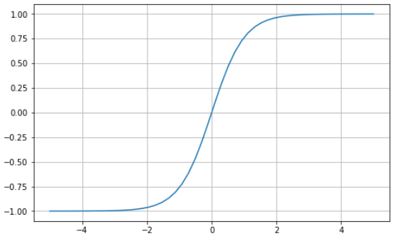
The hyperbolic tangent function (tanh) is similar to the sigmoid function in a sense: they share the “S” shaped curve characteristic. In contrast, the hyperbolic tangent function transforms the values between -1 and 1. This means inputs that are small (more negative) will be mapped closer to -1 (strongly negative) and 0 inputs will be mapped near 0.

Mathematical expression for tanh function

# tanh function in Python
import matplotlib.pyplot as plt
import numpy as npx = np.linspace(-5, 5, 50)
z = np.tanh(x)plt.subplots(figsize=(8, 5))
plt.plot(x, z)
plt.grid()plt.show()

Visual representation of the tanh function

Ian Goodfellow’s book, Deep Learning (P.195), states “…the hyperbolic tangent activation function typically performs better than the logistic sigmoid.” However, it suffers a similar fate to the sigmoid function, the vanishing gradient problem. It’s also computationally expensive due to its exponential operation.

How does the team at Uber manage to keep their data organized and their team united? Comet’s experiment tracking. Learn more from Uber’s Olcay Cirit.

Rectified Linear Unit (ReLU) Function

We tend to avoid using sigmoid and tanh functions when building neural networks with many layers due to the vanishing gradient problem. One solution could be to use the ReLU function which overcomes this problem and has become the default activation function for various neural networks.

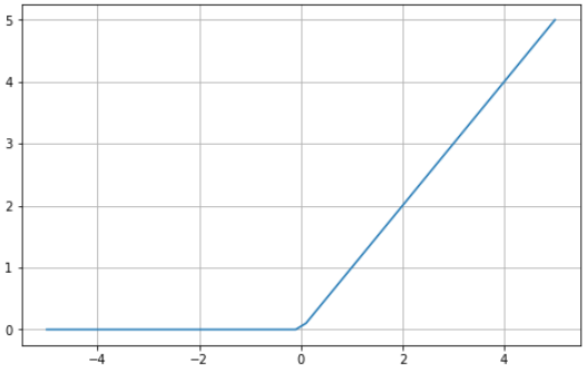
The ReLU activation function returns 0 if the input is 0 or less and returns the value provided as input directly if it’s greater than 0. Thus, the values range from 0 to infinity:

Mathematical expression for ReLU function

In Python, it looks as follows…

# ReLU in Python
import matplotlib.pyplot as plt
import numpy as npx = np.linspace(-5, 5, 50)
z = [max(0, i) for i in x]plt.subplots(figsize=(8, 5))
plt.plot(x, z)
plt.grid()plt.show()

Visual representation of ReLU function

Since the ReLU function looks and behaves mostly like a linear function, the neural network is much easier to optimize. It’s also very easy to implement.

Where the ReLU activation function suffers is when there are many negative values — they will all be outputted as 0. When this occurs, learning will be severely impacted and our model would be prohibited from properly learning complex patterns in the data. This is known as the dying ReLU problem. One solution to the dying ReLU problem is using Leaky ReLU.

Leaky ReLU Function

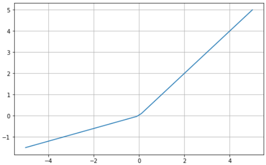
Leaky ReLU is an improvement on ReLU that attempts to combat the dying ReLU problem. Instead of defining the ReLU function as 0 for all negative values of x, it is defined as an extremely small linear component of x.

Mathematical expression for leaky ReLU function

The modification to the ReLU function alters the gradient for values equal to or less than 0 to be values that are non-zero. As a result, extremely small inputs would no longer encounter dead neurons.

Let’s see this in Python:

# leaky ReLU in Python
import matplotlib.pyplot as plt
import numpy as npx = np.linspace(-5, 5, 50)
z = [max((0.3*0), i) for i in x]plt.subplots(figsize=(8, 5))
plt.plot(x, z)
plt.grid()plt.show()

Visual representation of the Leaky ReLU function

Note: We typically set the α value to 0.01. Rarely ever is it set to 1 (or close to it) since that would make Leaky ReLU a linear function.

Exponential Linear Unit (ELU) Function

The Exponential Linear Unit (ELU) is an activation function for neural networks. In contrast to ReLUs, ELUs have negative values which allow them to push mean unit activations closer to zero like batch normalization but with lower computational complexity. Mean shifts toward zero speed up learning by bringing the normal gradient closer to the unit natural gradient because of a reduced bias shift effect. [Credit: PaperWithCode]

Mathematical expression for ELU function

# ELU function in Python
import matplotlib.pyplot as plt
from tensorflow.keras.activations import elux = np.linspace(-5, 5, 50)
z = elu(x, alpha=1)plt.subplots(figsize=(8, 5))
plt.plot(x, z)
plt.grid()plt.show()

Visual representation of the ELU function

Swish Function

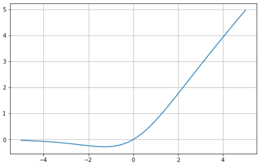
The swish function was announced as an alternative to ReLU by Google in 2017. It tends to perform better than ReLU in deeper networks, across a number of challenging datasets. This comes about after the authors showed that simply substituting ReLU activations with Swish functions improved the classification accuracy of ImageNet.

“Qfter performing analysis on ImageNet data, researchers from Google alleged that using the function as an activation function in artificial neural networks improves the performance, compared to ReLU and sigmoid functions. It is believed that one reason for the improvement is that the swish function helps alleviate the vanishing gradient problem during backpropagation.”
— [Source: Wikipedia]

One drawback of the swish function is that it’s computationally expensive in comparison to ReLU and its variants.

Mathematical expression for the swish function

# Swish function in Python
import matplotlib.pyplot as plt
import numpy as npx = np.linspace(-5, 5, 50)
z = x * (1/(1 + np.exp(-x)))plt.subplots(figsize=(8, 5))
plt.plot(x, z)
plt.grid()plt.show()

Visual representation of the Swish function

Many activation functions exist to help neural networks learn complex patterns in data. It’s common practice to use the same activation through all the hidden layers. For some activation functions, like the softmax activation function, it’s rare to see them used in hidden layers — we typically use the softmax function in the output layer when there are two or more labels.

The activation function you decide to use for your model may significantly impact the performance of the neural network. How to Choose an Activation Function for Deep Learning is a good article to learn more about choosing activation functions when building neural networks.

Thanks for reading.