Optimization plays a vital role in the development of machine learning and deep learning algorithms — without it, our model would not have the best design. The procedure refers to finding the set of input parameters or arguments to an objective function that results in the minimum or maximum output of the function — usually the minimum in a machine learning/deep learning context.
In this article, we are going to cover the top seven most common optimization methods used in deep learning.
#1 Gradient Descent
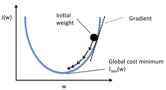
Getting a sound understanding of the inner workings of gradient descent is one of the best things you could do for your career in ML/DL. It’s one of the most popular optimization algorithms and comes up constantly in the field. Gradient descent is a first-order, iterative optimization method — first-order means we calculate only the first-order derivative.
To find the minimum of the function, steps are taken in proportion to the negative gradient of the function at its current point. The initial point on the function is random.

Gradient descent isn’t perfect though. An update to our parameters can only be made once we’ve iterated through the whole dataset which makes learning extremely slow when the data is large. Various adaptions to gradient descent were made to overcome this problem. They include mini-batch gradient descent and stochastic gradient descent.
#2 Momentum
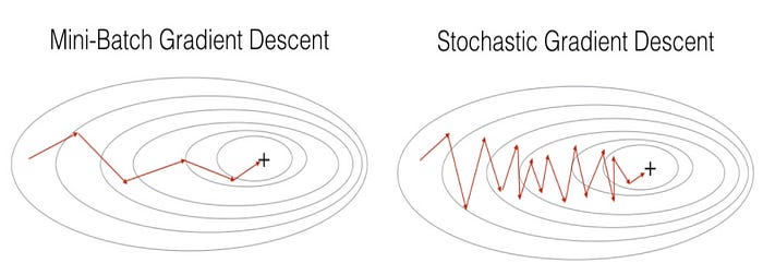
The two variations of gradient descent mentioned above — stochastic and mini-batch — oscillate as they step towards the minimum of the objective function. These oscillations occur because variance is introduced at each step since an update to the parameters is made after iterating through every n number of instances.

Momentum extends on gradient descent, hence we typically refer to it as gradient descent with momentum. The technique seeks to overcome the oscillation problem by adding history to the parameter update equation. The idea behind momentum is that with an understanding of the direction required to reach the minimum of the function faster, we can make our gradient steps move in that direction and reduce the oscillations in irrelevant directions.
The update parameter from the previous step, Vt−1, is added to the gradient step, ▽θJ(θ). How much information from historical steps depends on the value γ, and the step size is controlled by the learning rate, ŋ.

To update the parameter with momentum, we would use the following equation:

This adjustment applied to mini-batch and stochastic gradient descent will help to reduce oscillations in each gradient step which in turn would speed up convergence.
#3 Nesterov Accelerated Gradient (NAG)
Momentum-based optimization takes steps towards the minimum based on past steps, which reduces the oscillations we see in mini-batch and stochastic gradient descent. One problem arises when we use momentum is that we may miss the minimum value of the objective function. This is because, as we approach the minimum, the value for momentum is high.
“When the value of momentum is high while we are near to attain convergence, then the momentum actually pushes the gradient step high and it might miss out on the actual minimum value.” — Hands-on Deep Learning Algorithms with Python, P.101
Nesterov introduced an intelligent new method to help overcome this problem. The idea behind the method is to calculate the gradient of where the momentum would take us too, instead of calculating the gradient at the current position.
“Thus, before making gradient step with momentum and reaching a new position, if we understand which position the momentum will take us to, then we can avoid overshooting the minimum value.” — Hands-on Deep Learning Algorithms with Python, P.102
Upon learning that momentum is going to push us past the minimum value, we could reduce the speed of momentum to try to reach the minimum value.
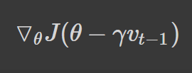
To identify the position in which we’d arrive at with momentum, we calculate the gradients with respect to the approximate position of where our next gradient step will be (the lookahead position):

We can rewrite the Vt equation presented in momentum as follows:

The parameter update step remains the same.
Join 16,000 of your colleagues at Deep Learning Weekly for the latest products, acquisitions, technologies, deep-dives and more.
#4 Adaptive Gradient (AdaGrad)
Adaptive gradient uses parameter-specific learning rates which are constantly adapted in accordance with how frequently a parameter update is made during training.
“Parameters that have frequent updates or high gradients will have a slower learning rate, while a parameter that has an infrequent update or small gradients will also have a slower learning rate. […] parameters that have infrequent updates implies that they are not trained enough, so we set a high learning rate for them, and parameters that have frequent updates implies they are trained enough, so we set their learning rate to a low value so we don’t overshoot the minimum.” — Hands-on Deep Learning Algorithms with Python, P.103
Let’s see how this looks from a mathematical standpoint. For simplicity’s sake, we are going to represent the gradient as g. Thus, the gradient of parameter, θi, at an iteration, t, can be represented as:

Our update equation can be rewritten as:

For each iteration, t, updating a parameter, θi, involves diving the learning rate by the sum of squares of all previous gradients of the parameter, θi (epsilon is added to avoid division by zero error):

When the sum of squares past gradients is a large value, our learning rate will be scaled to a smaller number. In contrast, if the value is low, the learning rate will be divided by a lower value, thus resulting in a higher learning rate.
#5 AdaDelta
Adadelta seeks to improve on the Agagrad optimization method. Recall that in Adagrad all the past squared gradients are summed together. This means that on every iteration the sum of the past squared gradients will increase, and when the squared past gradient value is high, we will be dividing the learning rate by a large number which causes the learning rate to decay. When the learning rate is a very small value, convergence will take longer.
“Instead of accumulating all past squared gradients, Adadelta restricts the window of accumulated past gradients to some fixed size w.” — An Overview of Gradient Descent Optimization Algorithms, Sebastien Ruder
To avoid the inefficient computation of squaring and storing gradients from the window, w, in each iteration, we take the exponentially decaying running average of gradients:

The γ we saw in momentum is similar to the one we see in this equation — it is used to decide how much information from the previous running average of gradients should be added. In Adadelta, it’s referred to as the exponential decaying rate.
Our final update equation is:

Note: See An Overview of Gradient Descent Optimization Algorithms, for the mathematical proof.
#6 RMSProp
RMSprop was also introduced to combat the decaying learning rate problem faced in Adagrad. We also use the exponentially decaying running average of the gradients:

We then divide the learning rate (0.9 is the recommended value), n, by this running average of gradients.

#7 Adaptive Moment Estimation (Adam)
Adam is probably the most popularly used optimization algorithm for neural networks. It combines RMSprop and momentum by not only storing the exponentially decaying average of past squared gradients (like we see in RMSprop and Adadelta), Vt, but also storing an exponentially decaying average of the past gradients, Mt, similar to momentum.
“Whereas momentum can be seen as a ball running down a slope, Adam behaves like a heavy ball with friction, which thus prefers flat minima in the error surface[15].” — An Overview of Gradient Descent Optimization Algorithms, Sebastien Ruder
We compute the decaying averages of the past, Mt, and past squared, Vt, gradients as follows:

The first moment (mean), Mt, and second moment (uncentered variance), Vt, are both estimates of the gradients — hence the name of the method.
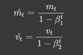
“When the initial estimates are set to 0, they remain very small, even after many iterations. This means that they would be biased towards 0, especially when β1 and β2 are close to 1.” — Hands-on Deep Learning Algorithms with Python, P.112
We can counteract the biases by computing the bias-corrected first and second-moment estimates:

Our final update parameter is given as:

In this article, we covered: Gradient descent, Momentum, NAG, Adagrad, Adadelta, RMSprop, and Adam optimization techniques. This is by no means an extensive list but serves as a good foundation for anyone interested in learning more about various optimizers used in deep learning. For a more in-depth look at the optimizers discussed, I highly recommend An Overview of Gradient Descent Optimization Algorithms, by Sebastien Ruder.