Introduction

Machine learning has expanded computers’ ability to understand images and extract different information from visual data. In this article, different computer vision tasks will be presented alongside explanations for how each has been tackled using machine learning.

A lot of machine learning research has been done in the field of computer vision throughout the last 3 decades. Different topics, tasks, and problems have been studied thoroughly; however, we’ll focus on the core problems of computer vision, and we’ll briefly present some of the more advanced hot topics in computer vision towards the end.

Classification

Image classification is the first computer vision task to be tackled by machine learning—in the 1950s, the perceptron algorithm was implemented in the Mark 1 Perceptron machine, which was used for image classification.

Although this algorithm was efficient for structured data problems, it could only perform well on trivial tasks such as classifying different geometric shapes. A few decades later, the SVM algorithm was introduced, which was able to tackle high-dimensional data with a minimum amount of samples, such as small image datasets.

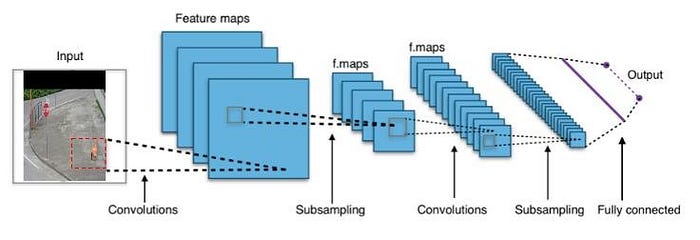
Finally, what has really revolutionized computer vision is the introduction of convolutional neural networks (CNNs) by Yann Lecun in his model LeNet, which was proven to be superior to other vision-based ML techniques in 2012, when AlexNet was the first CNN based model to win the famous ImageNet competition.

Problem Formulation

This part will be short since problem formulation is quite simple for classification. A classification problem generally involves classifying images into 2 or more classes.

In the case of using just two classes (ex: cat and no cat, text and background, etc.), the problem is known as a binary classification problem—for which, the last layer of the network will contain 1 neuron with a sigmoid activation function.

And in the case of using more than 2 classes (ex: digits, animals, vehicles, etc.), the problem is deemed a multi-class classification problem, for which the last layer will contain n neurons (n = Number Of Classes) with a softmax activation function.

Datasets and Benchmarks

The most famous dataset is the MNIST Handwritten Digits dataset, which has been used in the early age of computer vision and is still used as an introduction to image classification problems. Although this dataset has played an essential role in the development of computer vision, the task is considered trivial for the current state of the field and industry.

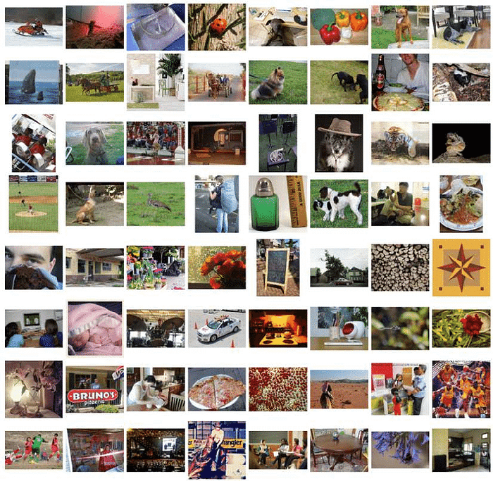
Currently, one of the most significant datasets is ImageNet, which consists of 1M samples of 1K classes of different animal species. This dataset is really important for image classification for two reasons.

First, It’s used as a benchmark for evaluating new network architectures through a yearly competition active from 2010 until 2017 and is still used for evaluating of new subsequent architectures. And second, it’s widely used to set pre-trained weights of other networks, as this dataset is so variant it can teach networks to detect important features in images that can be used in other computer vision tasks.

There are a lot of other datasets for image classification that have been used repeatedly through research—such as STL-10, CIFAR-10, and CIFAR-100—in a manner similar to ImageNet, but with less data and smaller image sizes.

As for medical research, a lot of datasets have been developed for different specific tasks such as ISIC, MURA, and DermNet. Medical datasets are harder to collect which is challenging for complicated tasks, as most of the time it’s not very feasible to collect large datasets when needed.

Significant Models

Although datasets can affect classification performance by presenting different variations in the data, the model architecture is also critical, as it affects the speed and the ability of the network to fit the data.

LeNet5 (LeCun et al.)

The LeNet architecture is considered the father of CNNs. It has a simple, shallow architecture, but it demonstrated the ability of convolution layers to learn good features from image data.

VGG (Simonyan, Zisserman)

This network showed that the deeper the network, the more it can learn. It has been proven efficient through experiments using different numbers of layers in the network. Although this network is considered quite small right now, it still can handle different tasks while using ImageNet for pre-training (weights are already available).

GoogleNet (Google) — Aka InceptionNet

In this work, they have successfully built an efficient network that can handle more complex tasks more efficiently, using a special building block (Inception Block) that contains 4 parallel paths, each containing different ConvLayers with different kernel sizes.

This technique enabled the network to utilize different kernel sizes in each layer while giving more weight to the more suitable kernel sizes. Another feature of this network is the use of intermediate classifiers, which could handle the problem of vanishing gradients better.

RestNet (Microsoft)

Using residual layers (link), this network attempts to solve the problem of depth— the deeper the network the harder it is to train. So by adding shortcut connections to the network that skip one or more layers, the network can perform identity mapping, which means it can’t perform worse than a network with fewer layers. Using this technique, they successfully trained a network 8 times deeper than VGG.

MobileNet (Google)

A move towards speed was made in this work, as researchers at Google used separable layers that decreased the number of computations required without affecting the model’s performance significantly. This technique made fitting convolutional neural networks on mobile devices much more achievable.

Object Localization and Detection

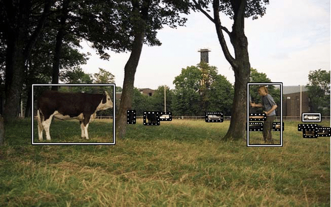
Object localization and detection is a computer vision problem in which, given an image, the algorithm has to decide the locations of one or more target objects, outputting bounding boxes for each that appears in the image or video frame.

This task is used heavily in different applications such as self-driving cars, robotics, augmented reality, and medical applications.

Problem Formulation

This problem can be formulated in different ways depending on the architecture being used. But generally, the network should output a class for each target object in the image using a sigmoid or a softmax activation function.

And to localize the object, the network outputs four variables representing the bounding box, which can be (x, y, w, h), with the x, y representing either the center or the top right corner of the bounding box.

Predicting the bounding box is considered a regression problem. Most of the algorithms require outputting another variable indicating whether an object exists in the selected area or not, as the output is produced for different parts of the image either via CNN implementation or using a sliding window.

Datasets and Benchmarks

Datasets for object localization and detection require more work than for image classification, as the bounding box is annotated around each target object in a given image. Let’s quick review a few datasets.

COCO, PASCAL, and ImageNet datasets are considered the main datasets used for evaluating new object detection architectures. They consist of large numbers of images of general objects like people, animals, cars, planes, etc., with annotations describing bounding boxes and classes for objects in the image. These datasets are also used for segmentation, which we’ll discuss in the next part.

Significant Models

Different techniques are used for building models for object detection. Some models rely on extracting region proposals and classifying each region separately, others use regions of interest (ROI) as an input to the model, while other approaches just use a single-shot network to handle the problem.

Sliding Window (Deformable Parts Models)

Some models have taken a sliding window approach to implement detection, in which a window slides through the image with a certain stride while inserting each block of the image into a classifier. The window is applied to different resolutions of the image to detect objects of different sizes. This approach is considered quite slow compared to the following examples, as the classification model is run once for every possible bounding box in the network.

R-CNN

The R-CNN approach relies on extracting region proposals via selective search. Then each region is wrapped and forwarded to a CNN pre-trained on ImageNet for feature extraction. Finally, the extracted features are forwarded to an SVM to classify each region. This approach has proved more accurate than sliding window approaches, but inference takes longer to process given the network’s separate stages.

R-CNN Improvements

Other architectures based on region proposals have followed the R-CNN approach. Fast R-CNN has better performance and speed relative to R-CNN, as it has merged feature extraction and classification into the same CNN. So the network has an image and multiple ROIs as input and it outputs a prediction for both the class and the bounding box for each ROI.

Faster R-CNN took it a step further by extracting ROIs through the network, which improved the accuracy and speed again. The reason behind this is that the network has more freedom to solve the problem. The weights can be updated throughout the network using end-to-end training, so the network has full control over ROIs and feature extraction.

YOLO

You only look once (YOLO) is a single-shot network that’s designed for optimal performance. It applies a CNN version of the sliding window approach by dividing the input image into an ss by reducing the image size through the network into ss cells with the same depths, where each cell represents a grid in the original image.

For each cell, there are B5 + C tensors representing B bounding box predictions and an array with length C representing the class. Because of this implementation detail, the network is limited in the number of nearby objects it can predict, as for each cell of the ss grid, it can only predict one class.

SSD

A single-shot multi-box detector can achieve a faster and more accurate performance than YOLO. It uses features from different levels in the network, which help detect objects with different sizes. Adding to that, the fast implementation of non-maximum suppression is essential for the network, as it outputs a large number of boxes for each image.

Segmentation

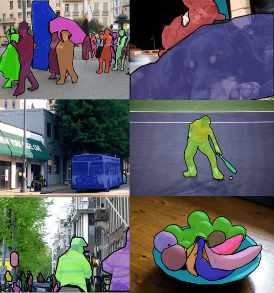
Image segmentation is used in various applications (medical, robotics, satellite imagery analysis, etc.) to not only understand the locations of objects in images and video frames, but to more precisely map the boundaries between different objects in the same image.

Problem Formulation

Image segmentation can be divided into two categories: semantic segmentation and instance segmentation, both of which require pixel-level labels.

For semantic segmentation, the solution requires objects’ pixels for each class of targets in the image to be labeled with the same value. Meanwhile, instance segmentation requires separating different instances of the same class by assigning their pixels different values. Some approaches handle the occlusion of objects so that the occluded part of the object is also represented.

Datasets and Benchmarks

Needless to say, segmentation datasets are of the most time-consuming datasets to build. Again, COCO and PASCAL datasets are two of the largest datasets for image segmentation, using general objects, as mentioned earlier.

Other datasets are built for more specific applications. For medical applications, there are a lot of datasets such as BraTS and Lits, which target tasks like tumor segmentation in different parts of the body and different types of diseases. Datasets like SpaceNet and the Agriculture-VisionDatabase consist of satellite images, which can have a variety of applications used for labeling large-scale things like streets, buildings, water bodies, etc.

Significant Models

For models handling segmentation problems, a different concept of ConvLayers should be used in addition to the traditional one—transpose convolution or deconvolution. Transpose convolution can output frames with larger spatial sizes than its input, which is needed for segmentation since the network infers the segmented image from features with smaller spatial size.

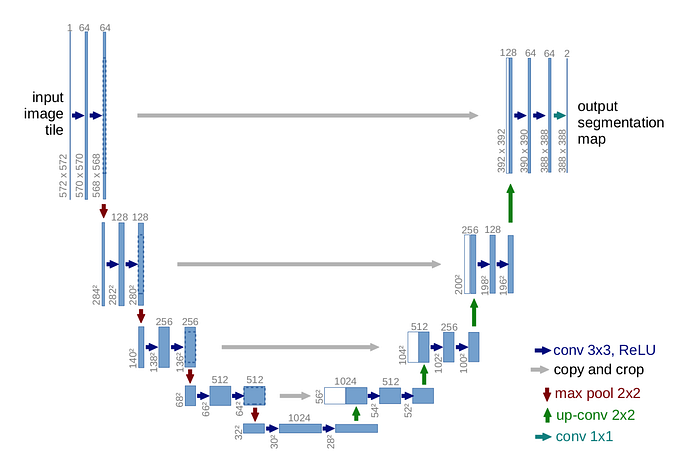
U-Net

The U-Net architecture is a full CNN that uses ConvLayers while reducing the spatial size and increasing the depth, and then the reverse by using transpose ConvLayers. Also, an important detail that affects the accuracy of the network is the forward propagation used between the early layers of the network and the later layers with the same spatial sizes, which can provide missing information due to the reduction of the window size.

Mask R-CNN

This network is an extension of Faster R-CNN, adding an extra branch predicting an object mask parallel to the bounding box prediction branch. In addition to this network being the state of the art for segmentation, it has been extended to perform several different tasks such as human pose estimation and rigid object pose estimation.

More Advanced Tasks

Computer vision can also tackle different tasks, which are a bit out of the scope of this article; however, we’ll offer simple descriptions for some examples of other tasks.

Data Generation

By learning the distribution of a dataset using approaches like GANs, we can generate new images that look real and can be used in new datasets. For example, by going to this website, you will see a new picture of a person that looks real—but has just generated by a CNN.

Domain Adaptation

Approaches like GANs and VAEs can be used to transform images from a source domain (street view in summer) to a target domain (street view in winter), which is very beneficial for generalizing networks’ performance on different tasks without annotating new data. This is also used for cool applications like deepfakes.

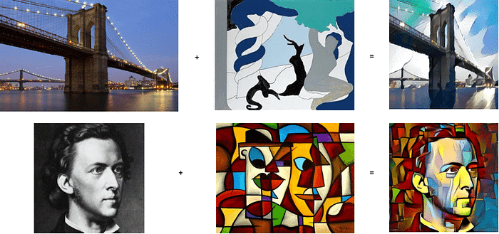
Neural Style Transfer

Another cool application of CNNs is neural style transfer, which uses a content image and a style image to output an image with the same content of the content image, but with the style of the style image. Using this, we can transform normal pictures into version that appear to be created by Van Gogh or Picasso.

Conclusion

In this survey of todays most essential machine learning-based computer vision techniques, we gave simple brief explanations of each topic to give the reader an overview of the range of possibilities, which can be a good way to start your journey with the field.