Build Multi-Index Advanced RAG Apps
Welcome to Lesson 12 of 12 in our free course series, LLM Twin: Building Your Production-Ready AI Replica. You’ll learn how to use LLMs, vector DVs, and LLMOps best practices to design, train, and deploy a production ready “LLM twin” of yourself. This AI character will write like you, incorporating your style, personality, and voice into an LLM. For a full overview of course objectives and prerequisites, start with Lesson 1.
Lessons
- An End-to-End Framework for Production-Ready LLM Systems by Building Your LLM Twin
- Your Content is Gold: I Turned 3 Years of Blog Posts into an LLM Training
- I Replaced 1000 Lines of Polling Code with 50 Lines of CDC Magic
- SOTA Python Streaming Pipelines for Fine-tuning LLMs and RAG — in Real-Time!
- The 4 Advanced RAG Algorithms You Must Know to Implement
- Turning Raw Data Into Fine-Tuning Datasets
- 8B Parameters, 1 GPU, No Problems: The Ultimate LLM Fine-tuning Pipeline
- The Engineer’s Framework for LLM & RAG Evaluation
- Beyond Proof of Concept: Building RAG Systems That Scale
- The Ultimate Prompt Monitoring Pipeline
- [Bonus] Build a scalable RAG ingestion pipeline using 74.3% less code
- [Bonus] Build Multi-Index Advanced RAG Apps
This article will teach you how to implement multi-index structures for building advanced RAG systems.
To implement our multi-index collections and queries, we will leverage Superlinked, a vector compute engine highly optimized for working with vector data, offering solutions for ingestion, embedding, storing and retrieval.
To better understand how Superlinked queries work, we will gradually present how to build a complex query that uses two vector indexes, adds filters based on the metadata extracted using an LLM, and returns only the top K most similar documents to reduce network I/O overhead.
Ultimately, we will dig into how Superlinked can help us implement and optimize various advanced RAG methods, such as query expansion, self-query, filtered vector search and rerank.
As this article is part of the LLM Twin course, before we start, here is some essential context you have to know to move along with this lesson (which you can read independently if you want to):
- In Lesson 11, we implemented the real-time RAG ingestion pipeline (using Bytewax) and server (using Superlinked).
- In Lesson 5, we presented 4 advanced RAG algorithms in depth and how to implement them.
Now, let’s move on to Lesson 12, our current lesson.
Table of Contents
- Exploring the multi-index RAG server
- Understanding the data ingestion pipeline
- Writing complex multi-index RAG queries using Superlinked
- Exploring the 4 advanced RAG optimization techniques
- Is Superlinked OP for building RAG and other vector-based apps?
🔗 Check out the code on GitHub [1] and support us with a ⭐️
1. Exploring the multi-index RAG server
We are using Superlinked to implement a powerful vector compute server. With just a few lines of code, we can implement a fully-fledged RAG application exposed as a REST API web server.
When using Superlinked, you declare your chunking, embedding and query strategy in a declarative way (similar to building a graph), making it extremely easy to implement an end-to-end workflow.
Let’s explore the core steps in how to define an RAG server using Superlinked ↓
First, you have to define the schema of your data, which in our case are the post, article, and repositories schemas:
 from superlinked import schema

@schema
class PostSchema:
  content: String
  platform: String
  ... # Other fields

@schema
class RepositorySchema:
  content: String
  platform: String
  ...

@schema
class ArticleSchema:
  content: String
  platform: String
  ...

post = PostSchema()
article = ArticleSchema()
repository = RepositorySchema()
You can quickly define an embedding space based on one or more schema attributes. The embedding space is made out of the following properties:
- the field to be embedded;
- a model used to embed the field.
For example, this is how you can define an embedding space for a piece of text, more precisely on the content of the article:
 from superlinked import TextSimilaritySpace, chunk

articles_space_content = TextSimilaritySpace(
    text=chunk(article.content, chunk_size=500, chunk_overlap=50),
    model=settings.EMBEDDING_MODEL_ID,
)
Notice that we also wrapped the article’s content field with the chunk() function that automatically chunks the text before embedding it.
The model can be any embedding model available on HuggingFace or SentenceTransformers. For example, we used the following MODEL_ID:
 from pydantic_settings import BaseSettings

class Settings(BaseSettings):
  EMBEDDING_MODEL_ID: str = "sentence-transformers/all-mpnet-base-v2"

  REDIS_HOSTNAME: str = "redis"
  REDIS_PORT: int = 6379

settings = Settings()
It also supports defining an embedding space for categorical variables, such as the article’s platform:
 from superlinked import CategoricalSimilaritySpace,

articles_space_plaform = CategoricalSimilaritySpace(
    category_input=article.platform,
    categories=["medium", "superlinked"],
    negative_filter=-5.0,
)
Along with text and categorical embedding spaces, Superlinked supports numerical and temporal variables:
- TextSimilaritySpace [2]
- CategoricalSimilaritySpace [5]
- RecencySpace [6]
- NumberSpace [7]
Multi-index structures
Now, we can combine the two embedding spaces defined above into a multi-index structure:
 from superlinked import Index

article_index = Index(
    [articles_space_content, articles_space_plaform],
    fields=[article.author_id],
)
The first attribute is a list with references to the text and categorical embedding spaces. At the same time, the fields parameter contains a list of all the fields to which we want to apply filters when querying the data. These steps will optimize retrieval and filter operations to run at low latencies.
Note that when defining an Index in Superlinked, we can add as many embedding spaces as we like that originate from the same schema, in our case, the ArticleSchema, where the minimum is one, and the maximum is all the schema fields.
…and, viola!
We defined a multi-index structure that supports weighted queries in just a few lines of code.
Using Superlinked and its embedding space and index architecture, we can easily index different data types (text, categorical, number, temporal) into a multi-index structure that offers tremendous flexibility in how we interact with the data.
The following section will show you how to query the multi-index collection defined above. But first, let’s wrap up with the Superlinked RAG server.
To do so, let’s define a connector to a Redis Vector DB:
 from superlinked import RedisVectorDatabase

vector_database = RedisVectorDatabase(
settings.REDIS_HOSTNAME,
settings.REDIS_PORT,
)
…and ultimately define a RestExecutor that wraps up everything from above into a REST API server:
 from superlinked import RestSource, RestExecutor, SuperlinkedRegistry

article_source = RestSource(article)
repository_source = RestSource(repository)
post_source = RestSource(post)

executor = RestExecutor(
    sources=[article_source, repository_source, post_source],
    indices=[article_index, repository_index, post_index],
    queries=[
        RestQuery(RestDescriptor("article_query"), article_query),
        RestQuery(RestDescriptor("repository_query"), repository_query),
        RestQuery(RestDescriptor("post_query"), post_query),
    ],
    vector_database=vector_database,
)
SuperlinkedRegistry.register(executor)
Based on all the queries defined in the RestExecutor class, Superlinked will automatically generate endpoints that can be called through HTTP requests.
In Lesson 11, we showed in more detail how the RAG Superlinked server works, how to set it up and how to interact with its query endpoints:
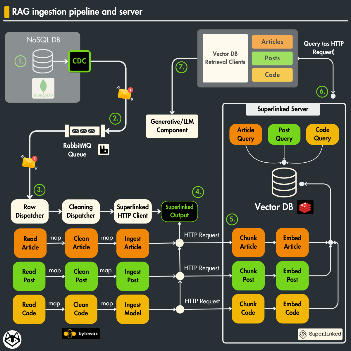
2. Understanding the data ingestion pipeline
Before we understand how to build queries for our multi-index collections, let’s have a quick refresher on how the vector DB is populated with article, post, and repository documents.
The data ingestion workflow is illustrated in Figure 2. During the LLM Twin course, we implemented a real-time data collection system in the following way:
- We crawl the data from the internet and store it in a MongoDB data warehouse.
- We use CDC to capture CRUD events on the database and send them as messages to a RabbitMQ queue.
- We use a Bytewax streaming engine to consume and clean the events from RabbitMQ in real time.
- Ultimately, the data is ingested into the Superlinked server through HTTP requests.
- As seen before, the Superlinked server does the heavy lifting, such as chunking, embedding, and loading all the ingested data into a Redis vector DB.
- We implemented a vector DB retrieval client that queries the data from Superlinked through HTTP requests.
- The vector DB retrieval will be used within the final RAG component, which generates the final response using the retrieved context and an LLM.
Note that whenever we crawl a new document from the Internet, we repeat steps 1–5, resulting in a vector DB synced with the external world in real-time.

If you want to see the full implementation of the steps above, you can always check out the rest of the course’s lessons for free, starting with Lesson 1.
But now that we have an intuition on how the Redis vector DB is populated with data used for RAG let’s see the true power of Superlinked and build some queries to retrieve data.
3. Writing complex multi-index RAG queries using Superlinked
Let’s take a look at the complete article query we want to define:
 article_query = (
Query(
article_index,
weights={
articles_space_content: Param("content_weight"),
articles_space_plaform: Param("platform_weight"),
},
)
.find(article)
.similar(articles_space_content.text, Param("search_query"))
.similar(articles_space_plaform.category, Param("platform"))
.filter(article.author_id == Param("author_id"))
.limit(Param("limit"))
)
If it seems like a lot, let’s break it into smaller pieces and start with the beginning.
What if we want to make a basic query that finds the most relevant articles solely based on the similarity between the query and the content of an article?
In the code snippet below, we define a query based on the article’s index to find articles that have the embedding of the content field most similar to the search query:
 article_query = (
    Query(article_index)
    .find(article)
    .similar(articles_space_content.text, Param("search_query"))
)
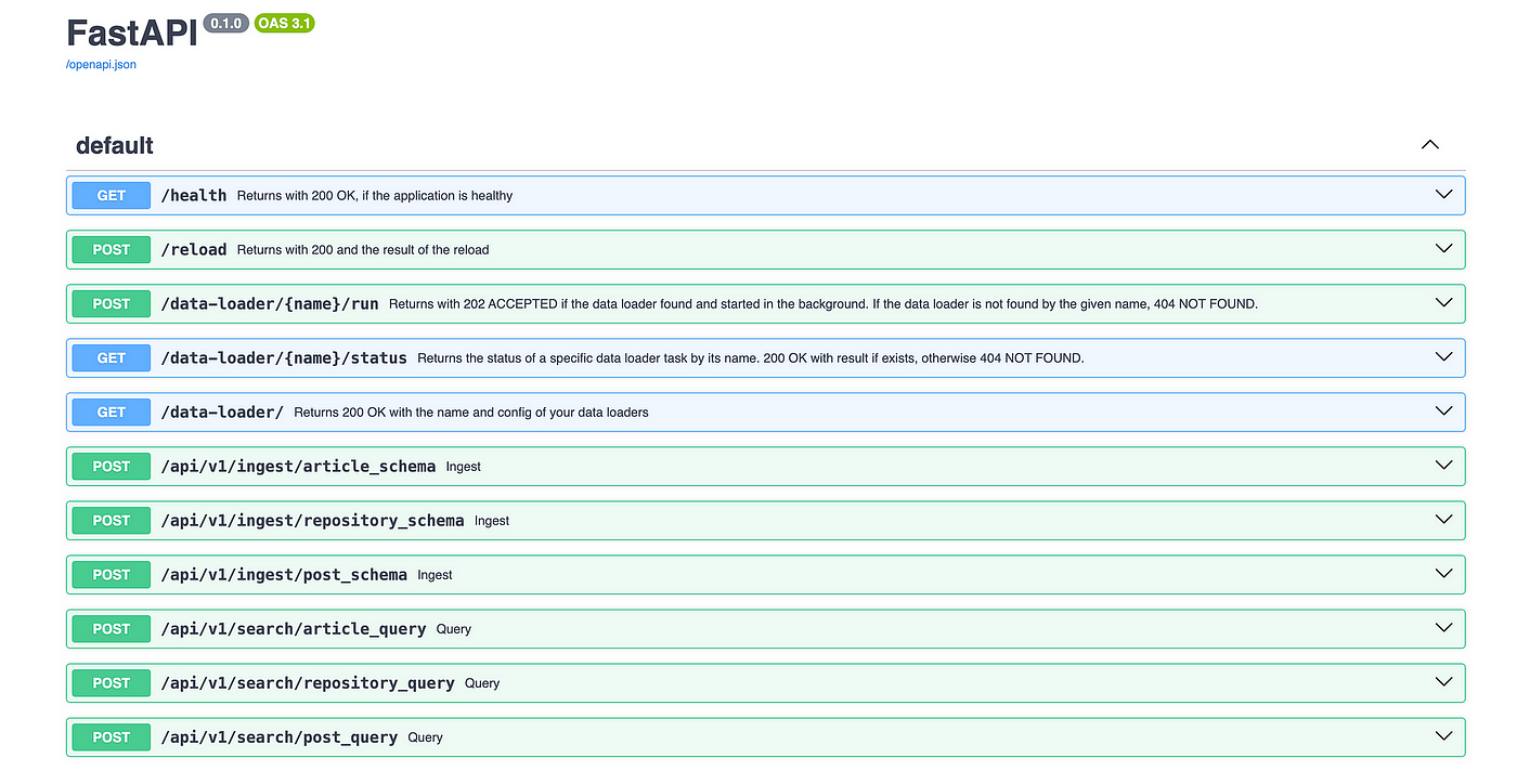
As seen in the Exploring the multi-index RAG server section, plugging this query into the RestExecutor class automatically creates an API endpoint accessible through POST HTTP requests.
In Figure 3, we can observe all the available endpoints automatically generated by Superlinked.
 import httpx

url=f"{base_url}/api/v1/search/article_query"
headers = {"Accept": "*/*", "Content-Type": "application/json"}

data = {
      "search_query": "Write me a post about Vector DBs and RAG.",
}
response = httpx.post(
    url, headers=headers, json=data, timeout=600
)
print(result["obj"])
As you can observe, all the attributes wrapped by the Param() class within the query are expected as parameters within the POST request, such as the Param(“search_query”), which represents the user’s query.
Quite intuitive, right?
Now… What happens behind the scenes?
After the endpoint is called, the Superlinked server processes the search query based on the articles_space_content embedding text space, which defines how to chunk and embed a text.
Thus, that will happen to the search query: it will chunk and embed it.
Using the computed query embedding, it will search the vector space based on the article’s content and retrieve the most similar documents:
 articles_space_content = TextSimilaritySpace(
    text=chunk(article.content, chunk_size=500, chunk_overlap=50),
    model="sentence-transformers/all-mpnet-base-v2",
)
Multi-index query
Now that we understand the basics of how a Superlinked query works, let’s add another layer of complexity and create a multi-index query based on the article’s content and platform:
 article_query = (
    Query(
        article_index,
        weights={
            articles_space_content: Param("content_weight"),
            articles_space_plaform: Param("platform_weight"),
        },
    )
    .find(article)
    .similar(articles_space_content.text, Param("search_query"))
    .similar(articles_space_plaform.category, Param("platform"))
)
We added two things.
The first one is another similar() function call, which configures the other embedding space we should use for the query, which is articles_space_plaform.
Now, when making a query, Superlinked will use the embedding of both fields to search for relevant information:
- the search query
- the article’s platforms
But how do we configure which one is more important?
Here, the second thing that we added kicks in, which is the weights parameter within the Query(weights={…}) class.
Using the weights dictionary, we can add different weights per index to configure the importance of each within a particular query.
Let’s better understand this with an example:
 data = {
    "search_query": "Write me a post about Vector DBs and RAG.",
    "platform": "medium",
    "content_weight": 0.9, # 90%
    "platform_weight": 0.1, # 10%
}
response = httpx.post(
    url, headers=self.headers, json=data, timeout=self.timeout
)
In the previous example, we set the content weight to 90% and the platform’s to 10%, which means that the article’s content will most impact our query but still favor articles from the same platform.
By playing with these weights, we tweak the impact of each index in our query.
Now, let’s add the last final pieces of the query, which are the filter() and the limit() functions:
 article_query = (
    Query(
        article_index,
        weights={
            articles_space_content: Param("content_weight"),
            articles_space_plaform: Param("platform_weight"),
        },
    )
    .find(article)
    .similar(articles_space_content.text, Param("search_query"))
    .similar(articles_space_plaform.category, Param("platform"))
    .filter(article.author_id == Param("author_id"))
    .limit(Param("limit"))
)
The author_id filter helps us retrieve documents only from a specific author, while the limit function controls how many items we want to retrieve.
For example, if we find 10 similar articles but the limit is set to 3, the Superlinked server will always return a maximum of 3 documents. Thus reducing network I/O between the server and client:
 data = {
    "search_query": "Write me a post about Vector DBs and RAG.",
    "platform": "medium",
    "content_weight": 0.9, # 90%
    "platform_weight": 0.1, # 10%
    "author_id": 145,
    "limit": 3,
}
response = httpx.post(
    url, headers=self.headers, json=data, timeout=self.timeout
)
That’s it! We can further optimize our retrieval step by experimenting with other multi-index configurations and weights.
4. Exploring the 4 advanced RAG optimization techniques
In Lesson 5, we explored 4 popular advanced RAG techniques to improve the accuracy of our generative AI system.
As a quick reminder, there are 3 main types of advanced RAG techniques:
- Pre-retrieval optimization [ingestion]: tweak how you create the chunks
- Retrieval optimization [retrieval]: improve the queries to your vector DB
- Post-retrieval optimization [retrieval]: process the retrieved chunks to filter out the noise
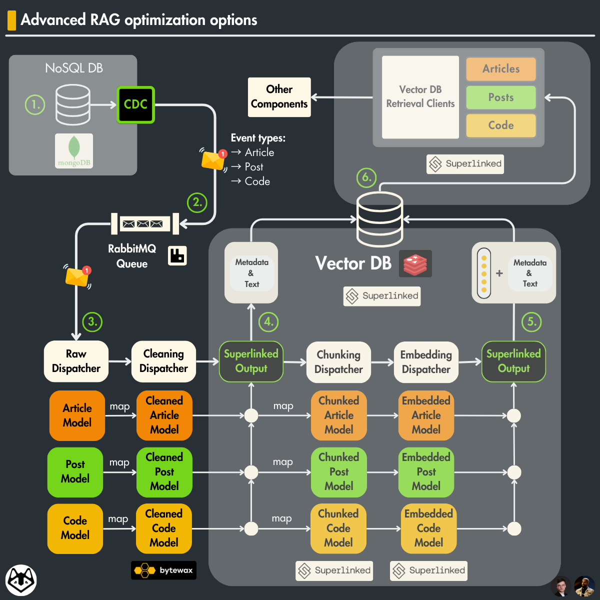
Figure 4: Advanced RAG optimization options
Now, let’s explore the 4 methods initially implemented in Lesson 5 and understand how they can be integrated into our new architecture:
- Query expansion (retrieval)
- Self query (retrieval)
- Filtered vector search (retrieval)
- Rerank (post-retrieval)
By incorporating these 4 advanced RAG optimization techniques, we will better understand where Superlinked shines most.
Important > On optimizing the ingestion side, Superlinked handled everything from chunking, embedding, and loading into a vector DB, detailed in Lesson 11.
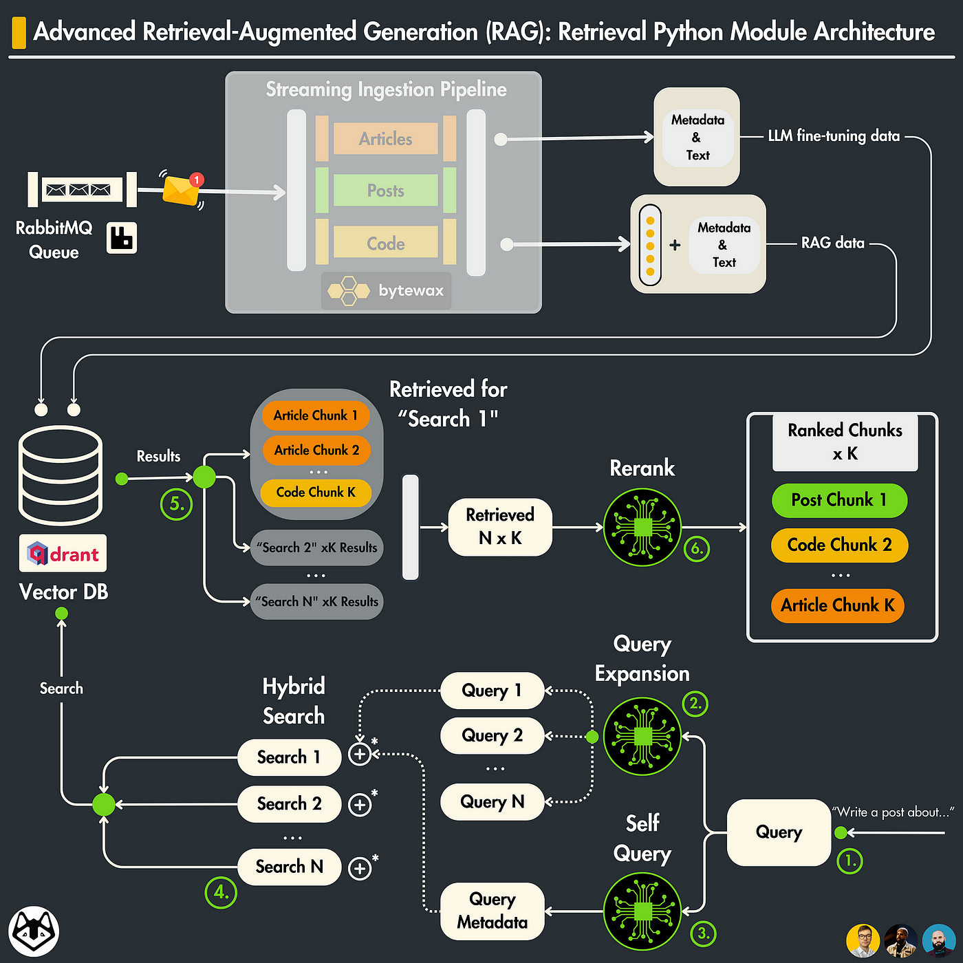
Query expansion (retrieval)
To implement query expansion, you use an LLM to generate multiple queries based on your initial user’s query.
These queries will contain multiple perspectives of the initial query.
Thus, when embedded, they hit different areas of your embedding space that are still relevant to our initial question.
Does Superlinked help here? Not really, as you have to expand your query before calling Superlinked.
Self query (retrieval)
What if you could extract the tags within the query and use them along your vector search?
That is what self-query is all about!
You use an LLM to extract critical metadata fields for your business use case (e.g., tags, author ID, number of comments, likes, shares, etc.)
In our custom solution, we are extracting just the author ID. Thus, a zero-shot prompt engineering technique will do the job.
Does Superlinked help here? Unfortunately, no, as you have to apply a self-query before calling the Superlinked server.
But… self-queries work hand-in-hand with vector filter searches, which we will explain in the next section.
Filtered vector search (retrieval)
This is a fancy name for applying a standard filter on your metadata before (or after) doing your vector search, hence “Filtered vector search.”
Does Superlinked help here? Yes! This is where Superlinked shines, allowing you to quickly index data structured on fields other than your vector index (or multi-index).
 article_index = Index(
    [articles_space_content, articles_space_plaform],
    fields=[article.author_id],
)

article_query = (
    Query(article_index)
    ...
    .filter(article.author_id == Param("author_id"))
)
Thus, you can implement optimal queries tailored to your data with a few lines of code.
Rerank (post-retrieval)
Rerank is used to filter out the noise from your retrieved documents.
For example, you retrieved N documents from your vector DB using Superlinked. However, you want to be prudent about your context size, so you use a rerank model to score the relevancy of all the retrieved documents relative to your query.
Then, based on the rerank score, you pick only the top K (where K < N) documents as your final items to build up the context.
Does Superlinked help here? Unfortunately, it doesn’t support cross-encoder models [3] for reranking.
But they are just at the beginning of their journey. Supporting reranking makes a lot of sense. Thus, we speculate that they will add it along with other functionality that optimizes the retrieval component of an RAG system (or other AI application that works with embeddings).
In this article, we briefly discussed the 4 advanced RAG methods implemented in our course. Check out Lesson 5 for a detailed explanation of each method.
5. Is Superlinked OP for building RAG and other vector-based apps?
Superlinked has incredible potential to build scalable vector servers to ingest and retrieve your data based on operations between embeddings.
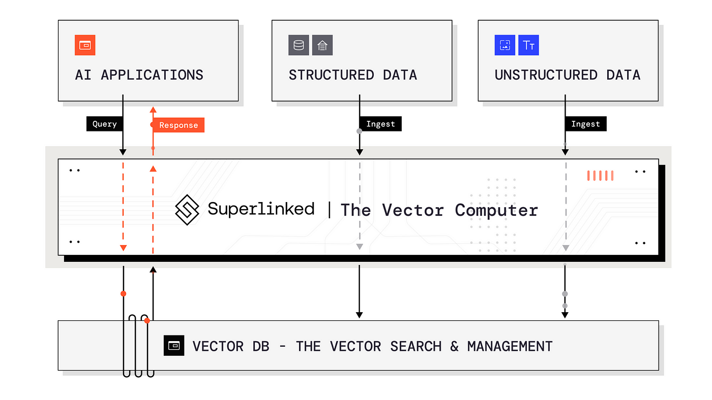
As you’ve seen in Lesson 11 and Lesson 12, in just a few lines of code, we’ve:
- implemented clean and modular schemas for your data;
- chunked and embedded the data;
- added embedding support for multiple data types (text, categorical, numerical, temporal);
- implemented multi-index collections and queries, allowing us to optimize our retrieval step;
- connectors for multiple vector DBs (Redis, MongoDB, etc.)
- optimized filtered vector search.
The truth is that Superlinked is still a young Python framework.
But as it grows, it will become more stable and introduce even more features, such as rerank, making it an excellent choice for implementing your vector search layer.
If you are curious, check out Superlinked to learn more about them.
Conclusion
Within this article, you’ve learned how to implement multi-index collections and queries for advanced RAG using Superlinked.
After to better understand how Superlinked queries work, we gradually presented how to build a complex query that:
- uses two vector indexes;
- adds filters based on the metadata extracted with an LLM;
- returns only the top K elements to reduce network I/O overhead.
Ultimately, we looked into how Superlinked can help us implement and optimize various advanced RAG methods, such as query expansion, self-query, filtered vector search and rerank.
With this, we’ve wrapped up the LLM Twin open-source course. We hope you enjoyed it and it brought value to your LLM & RAG skills.
The next step is to clone our LLM Twin GitHub repository [1] and run everything yourself to get the most out of these series.
References
Literature
[1] Your LLM Twin Course — GitHub Repository (2024), Decoding ML’s GitHub Organization
Images
If not otherwise stated, all images are created by the author.
